C World Map

In this chapter, we study the topic of drawing world maps using ggplot2.

Using a map data in data.frame to apply geom_map or geom_polygon is possible. However, recently, we can obtain a map data in simple feature (sf) format, ad ggplot2 includes a special geom called geom_sf to draw more complex data.

C.1 Setup

library(tidyverse)
#> ── Attaching core tidyverse packages ──── tidyverse 2.0.0 ──
#> ✔ dplyr     1.1.3     ✔ readr     2.1.4
#> ✔ forcats   1.0.0     ✔ stringr   1.5.0
#> ✔ ggplot2   3.4.4     ✔ tibble    3.2.1
#> ✔ lubridate 1.9.3     ✔ tidyr     1.3.0
#> ✔ purrr     1.0.2     
#> ── Conflicts ────────────────────── tidyverse_conflicts() ──
#> ✖ dplyr::filter() masks stats::filter()
#> ✖ dplyr::lag()    masks stats::lag()
#> ℹ Use the conflicted package (<http://conflicted.r-lib.org/>) to force all conflicts to become errors
library(sf)
#> Linking to GEOS 3.11.0, GDAL 3.5.3, PROJ 9.1.0; sf_use_s2()
#> is TRUE
library(showtext)
#> Loading required package: sysfonts
#> Loading required package: showtextdb
showtext_auto()

We will use income level data with the iso2c code of each country obtained using WDIcache().

wdi_cache <- read_rds("./data/wdi_cache.RData")

wdi_cache$country %>% as_tibble() %>% glimpse()
#> Rows: 299
#> Columns: 9
#> $ iso3c     <chr> "ABW", "AFE", "AFG", "AFR", "AFW", "AGO"…
#> $ iso2c     <chr> "AW", "ZH", "AF", "A9", "ZI", "AO", "AL"…
#> $ country   <chr> "Aruba", "Africa Eastern and Southern", …
#> $ region    <chr> "Latin America & Caribbean", "Aggregates…
#> $ capital   <chr> "Oranjestad", "", "Kabul", "", "", "Luan…
#> $ longitude <chr> "-70.0167", "", "69.1761", "", "", "13.2…
#> $ latitude  <chr> "12.5167", "", "34.5228", "", "", "-8.81…
#> $ income    <chr> "High income", "Aggregates", "Low income…
#> $ lending   <chr> "Not classified", "Aggregates", "IDA", "…

wdi_income <- wdi_cache$country %>% 
  filter(region != "Aggregates") %>%
  select(iso2c, income) %>% 
  drop_na(iso2c) %>%
  mutate(income = factor(income, levels = c("High income", "Upper middle income", "Lower middle income", "Low income", "Not classified", NA))) 
glimpse(wdi_income)
#> Rows: 218
#> Columns: 2
#> $ iso2c  <chr> "AW", "AF", "AO", "AL", "AD", "AE", "AR", "…
#> $ income <fct> High income, Low income, Lower middle incom…

C.1.1 `geom_sf`

See also, coord_sf, geom_sf_label, geom_sf_text, stat_sf.

This set of geom, stat, and coord are used to visualise simple feature (sf) objects. For simple plots, you will only need geom_sf() as it uses stat_sf() and adds coord_sf() for you. geom_sf() is an unusual geom because it will draw different geometric objects depending on what simple features are present in the data: you can get points, lines, or polygons. For text and labels, you can use geom_sf_text() and geom_sf_label().

geom_sf(
  mapping = aes(),
  data = NULL,
  stat = "sf",
  position = "identity",
  na.rm = FALSE,
  show.legend = NA,
  inherit.aes = TRUE,
  ...
)

C.2 Natural Earth Data

https://www.naturalearthdata.com

Get natural earth world country polygons

Manual: https://cran.r-project.org/web/packages/rnaturalearth/rnaturalearth.pdf

C.2.1 `ne_countries`

library(rnaturalearth)
#> Support for Spatial objects (`sp`) will be deprecated in {rnaturalearth} and will be removed in a future release of the package. Please use `sf` objects with {rnaturalearth}. For example: `ne_download(returnclass = 'sf')`
library(rnaturalearthdata)
#> 
#> Attaching package: 'rnaturalearthdata'
#> The following object is masked from 'package:rnaturalearth':
#> 
#>     countries110

ne_countries(
  scale = 110,
  type = "countries",
  continent = NULL,
  country = NULL,
  geounit = NULL,
  sovereignty = NULL,
  returnclass = c("sp", "sf")
)

C.2.1.1 Arguments

scale: scale of map to return, one of 110, 50, 10 or ‘small’, ‘medium’, ‘large’
type: country type, one of ‘countries’, ‘map_units’, ‘sovereignty’, ‘tiny_countries’
continent: a character vector of continent names to get countries from.
country: a character vector of country names.
geounit: a character vector of geounit names.
sovereignty: a character vector of sovereignty names.
returnclass: ‘sp’ default or ‘sf’ for Simple Features

C.2.1.2 Examples

There are three scales. Add returnclass = "sf" as an option to obtain data in sf format.

ne_countries(scale = "large", returnclass = "sf") %>%
  ggplot() +   geom_sf()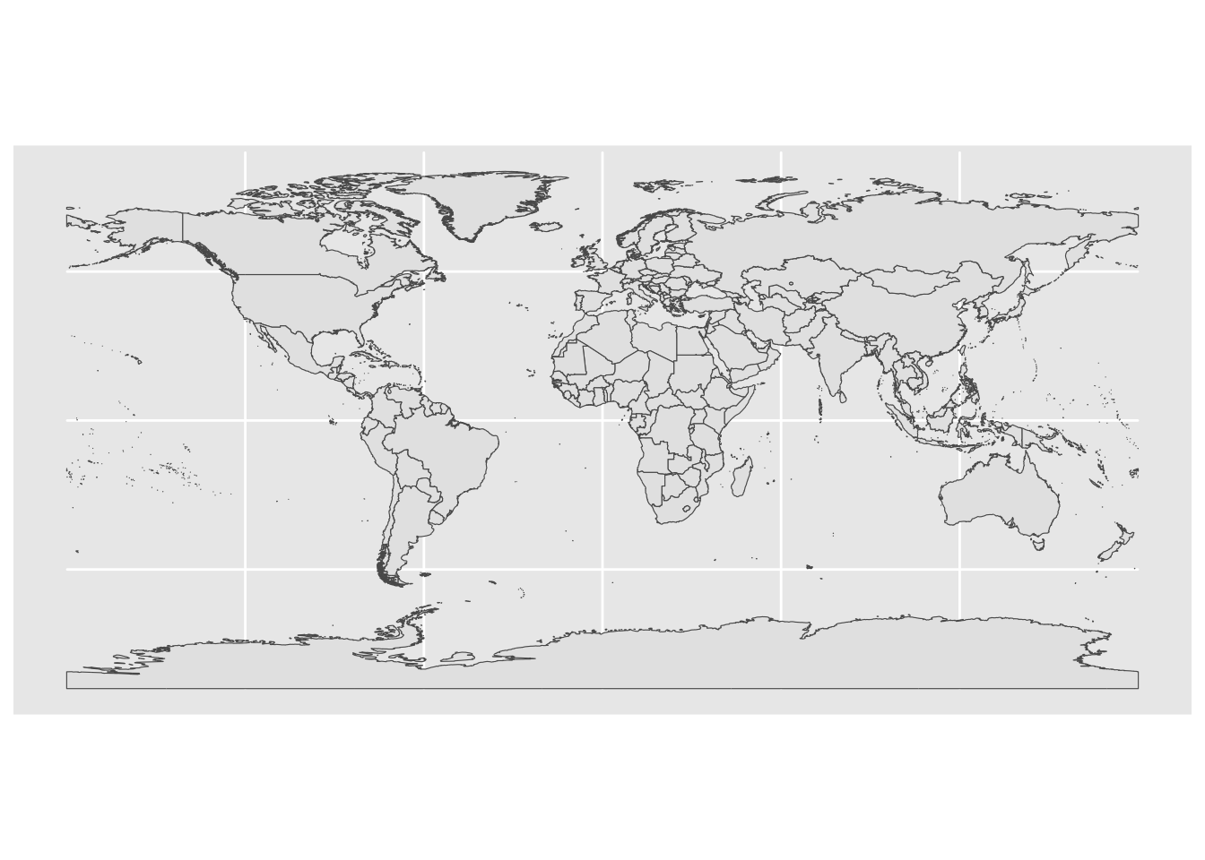

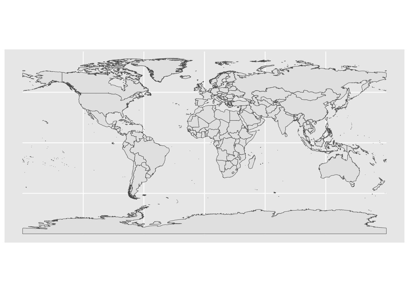
ne_countries(scale = "small", returnclass = "sf") %>%
  ggplot() +   geom_sf()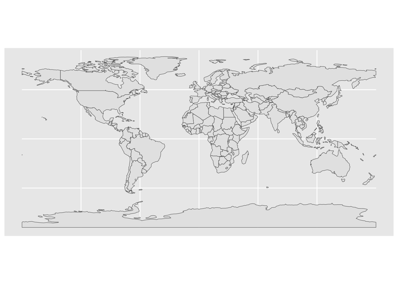

We will use medium scale data in the following.

ne_world <- ne_countries(scale = "medium", returnclass = "sf")

glimpse(ne_world)
#> Rows: 241
#> Columns: 64
#> $ scalerank  <int> 3, 1, 1, 1, 1, 3, 3, 1, 1, 1, 3, 1, 5, …
#> $ featurecla <chr> "Admin-0 country", "Admin-0 country", "…
#> $ labelrank  <dbl> 5, 3, 3, 6, 6, 6, 6, 4, 2, 6, 4, 4, 5, …
#> $ sovereignt <chr> "Netherlands", "Afghanistan", "Angola",…
#> $ sov_a3     <chr> "NL1", "AFG", "AGO", "GB1", "ALB", "FI1…
#> $ adm0_dif   <dbl> 1, 0, 0, 1, 0, 1, 0, 0, 0, 0, 1, 0, 1, …
#> $ level      <dbl> 2, 2, 2, 2, 2, 2, 2, 2, 2, 2, 2, 2, 2, …
#> $ type       <chr> "Country", "Sovereign country", "Sovere…
#> $ admin      <chr> "Aruba", "Afghanistan", "Angola", "Angu…
#> $ adm0_a3    <chr> "ABW", "AFG", "AGO", "AIA", "ALB", "ALD…
#> $ geou_dif   <dbl> 0, 0, 0, 0, 0, 0, 0, 0, 0, 0, 0, 0, 0, …
#> $ geounit    <chr> "Aruba", "Afghanistan", "Angola", "Angu…
#> $ gu_a3      <chr> "ABW", "AFG", "AGO", "AIA", "ALB", "ALD…
#> $ su_dif     <dbl> 0, 0, 0, 0, 0, 0, 0, 0, 0, 0, 0, 0, 0, …
#> $ subunit    <chr> "Aruba", "Afghanistan", "Angola", "Angu…
#> $ su_a3      <chr> "ABW", "AFG", "AGO", "AIA", "ALB", "ALD…
#> $ brk_diff   <dbl> 0, 0, 0, 0, 0, 0, 0, 0, 0, 0, 0, 0, 0, …
#> $ name       <chr> "Aruba", "Afghanistan", "Angola", "Angu…
#> $ name_long  <chr> "Aruba", "Afghanistan", "Angola", "Angu…
#> $ brk_a3     <chr> "ABW", "AFG", "AGO", "AIA", "ALB", "ALD…
#> $ brk_name   <chr> "Aruba", "Afghanistan", "Angola", "Angu…
#> $ brk_group  <chr> NA, NA, NA, NA, NA, NA, NA, NA, NA, NA,…
#> $ abbrev     <chr> "Aruba", "Afg.", "Ang.", "Ang.", "Alb."…
#> $ postal     <chr> "AW", "AF", "AO", "AI", "AL", "AI", "AN…
#> $ formal_en  <chr> "Aruba", "Islamic State of Afghanistan"…
#> $ formal_fr  <chr> NA, NA, NA, NA, NA, NA, NA, NA, NA, NA,…
#> $ note_adm0  <chr> "Neth.", NA, NA, "U.K.", NA, "Fin.", NA…
#> $ note_brk   <chr> NA, NA, NA, NA, NA, NA, NA, NA, NA, NA,…
#> $ name_sort  <chr> "Aruba", "Afghanistan", "Angola", "Angu…
#> $ name_alt   <chr> NA, NA, NA, NA, NA, NA, NA, NA, NA, NA,…
#> $ mapcolor7  <dbl> 4, 5, 3, 6, 1, 4, 1, 2, 3, 3, 4, 4, 1, …
#> $ mapcolor8  <dbl> 2, 6, 2, 6, 4, 1, 4, 1, 1, 1, 5, 5, 2, …
#> $ mapcolor9  <dbl> 2, 8, 6, 6, 1, 4, 1, 3, 3, 2, 1, 1, 2, …
#> $ mapcolor13 <dbl> 9, 7, 1, 3, 6, 6, 8, 3, 13, 10, 1, NA, …
#> $ pop_est    <dbl> 103065, 28400000, 12799293, 14436, 3639…
#> $ gdp_md_est <dbl> 2258.0, 22270.0, 110300.0, 108.9, 21810…
#> $ pop_year   <dbl> NA, NA, NA, NA, NA, NA, NA, NA, NA, NA,…
#> $ lastcensus <dbl> 2010, 1979, 1970, NA, 2001, NA, 1989, 2…
#> $ gdp_year   <dbl> NA, NA, NA, NA, NA, NA, NA, NA, NA, NA,…
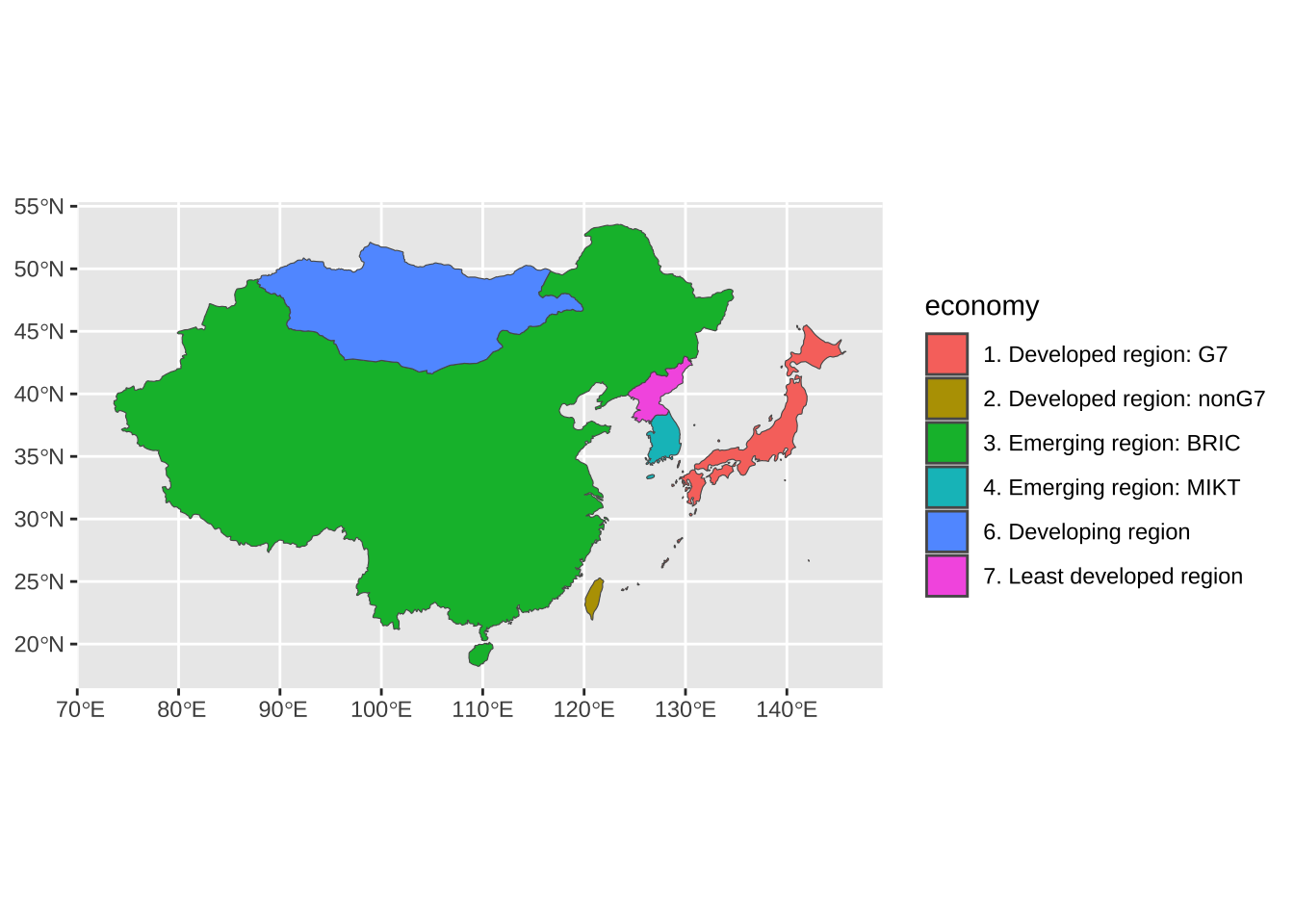
#> $ economy    <chr> "6. Developing region", "7. Least devel…
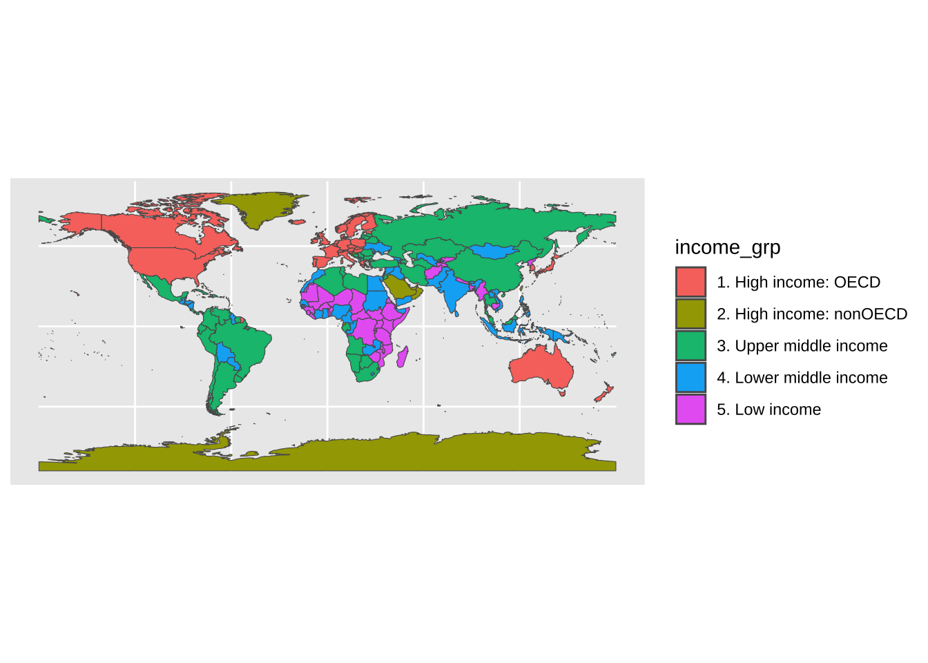
#> $ income_grp <chr> "2. High income: nonOECD", "5. Low inco…
#> $ wikipedia  <dbl> NA, NA, NA, NA, NA, NA, NA, NA, NA, NA,…
#> $ fips_10    <chr> NA, NA, NA, NA, NA, NA, NA, NA, NA, NA,…
#> $ iso_a2     <chr> "AW", "AF", "AO", "AI", "AL", "AX", "AD…
#> $ iso_a3     <chr> "ABW", "AFG", "AGO", "AIA", "ALB", "ALA…
#> $ iso_n3     <chr> "533", "004", "024", "660", "008", "248…
#> $ un_a3      <chr> "533", "004", "024", "660", "008", "248…
#> $ wb_a2      <chr> "AW", "AF", "AO", NA, "AL", NA, "AD", "…
#> $ wb_a3      <chr> "ABW", "AFG", "AGO", NA, "ALB", NA, "AD…
#> $ woe_id     <dbl> NA, NA, NA, NA, NA, NA, NA, NA, NA, NA,…
#> $ adm0_a3_is <chr> "ABW", "AFG", "AGO", "AIA", "ALB", "ALA…
#> $ adm0_a3_us <chr> "ABW", "AFG", "AGO", "AIA", "ALB", "ALD…
#> $ adm0_a3_un <dbl> NA, NA, NA, NA, NA, NA, NA, NA, NA, NA,…
#> $ adm0_a3_wb <dbl> NA, NA, NA, NA, NA, NA, NA, NA, NA, NA,…
#> $ continent  <chr> "North America", "Asia", "Africa", "Nor…
#> $ region_un  <chr> "Americas", "Asia", "Africa", "Americas…
#> $ subregion  <chr> "Caribbean", "Southern Asia", "Middle A…
#> $ region_wb  <chr> "Latin America & Caribbean", "South Asi…
#> $ name_len   <dbl> 5, 11, 6, 8, 7, 5, 7, 20, 9, 7, 14, 10,…
#> $ long_len   <dbl> 5, 11, 6, 8, 7, 13, 7, 20, 9, 7, 14, 10…
#> $ abbrev_len <dbl> 5, 4, 4, 4, 4, 5, 4, 6, 4, 4, 9, 4, 7, …
#> $ tiny       <dbl> 4, NA, NA, NA, NA, 5, 5, NA, NA, NA, 3,…
#> $ homepart   <dbl> NA, 1, 1, NA, 1, NA, 1, 1, 1, 1, NA, 1,…
#> $ geometry   <MULTIPOLYGON [°]> MULTIPOLYGON (((-69.89912 …

The last column is the geometry which contains map data in multi-polygon format.

ne_world %>% ggplot() + geom_sf()

This map data comes with various information.

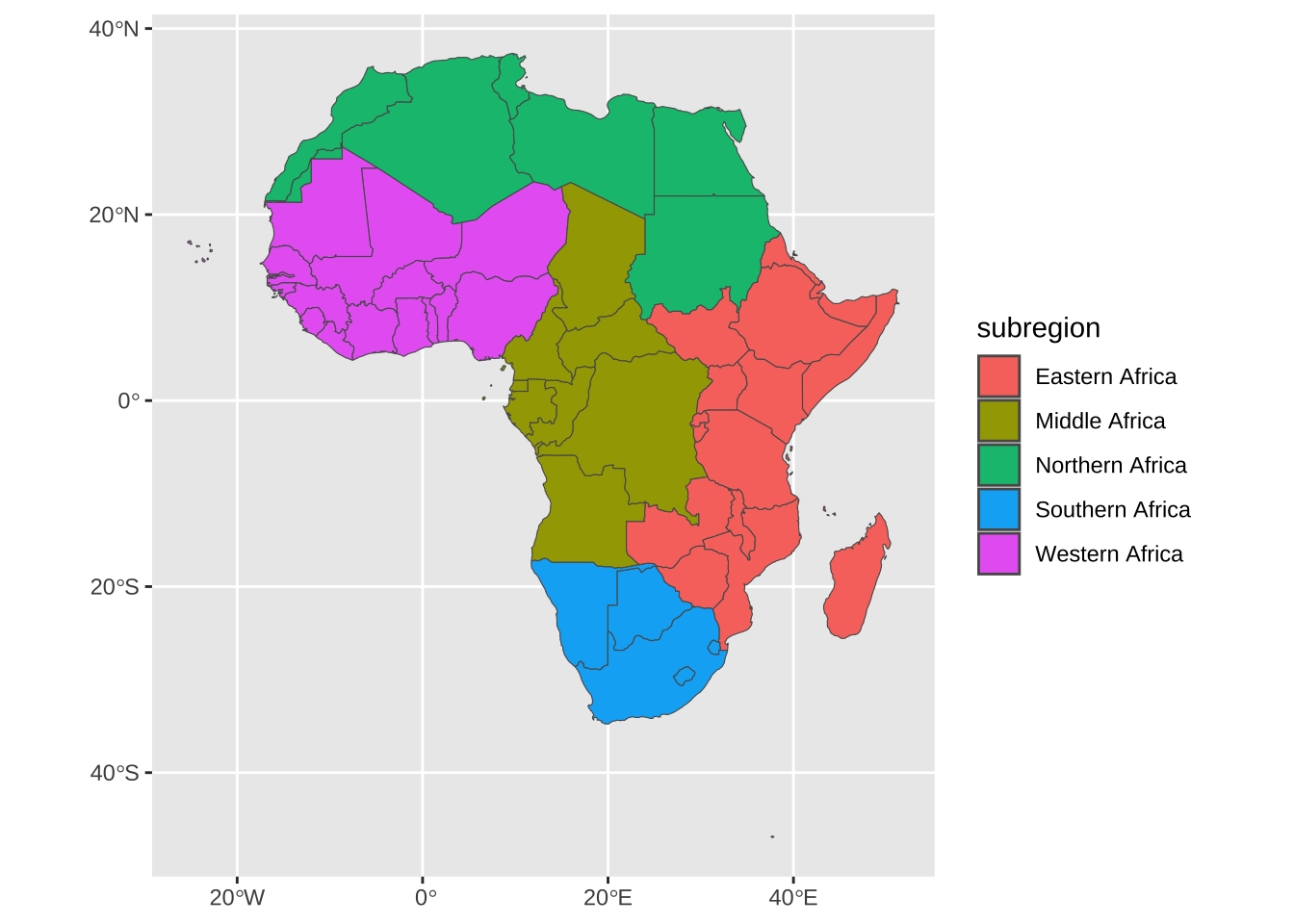
ne_world %>% ggplot() + geom_sf(aes(fill = income_grp))

You can specify a ‘continent’, a ‘region_un’, a ‘subregion’ or ‘region_wb’.

ne_world %>% as_tibble() %>% distinct(continent) %>% pull()
#> [1] "North America"           "Asia"                   
#> [3] "Africa"                  "Europe"                 
#> [5] "South America"           "Oceania"                
#> [7] "Antarctica"              "Seven seas (open ocean)"

ne_world %>% as_tibble() %>% distinct(region_un) %>% pull()
#> [1] "Americas"                "Asia"                   
#> [3] "Africa"                  "Europe"                 
#> [5] "Oceania"                 "Antarctica"             
#> [7] "Seven seas (open ocean)"

ne_world %>% as_tibble() %>% distinct(subregion) %>% pull()
#>  [1] "Caribbean"                 "Southern Asia"            
#>  [3] "Middle Africa"             "Southern Europe"          
#>  [5] "Northern Europe"           "Western Asia"             
#>  [7] "South America"             "Polynesia"                
#>  [9] "Antarctica"                "Australia and New Zealand"
#> [11] "Seven seas (open ocean)"   "Western Europe"           
#> [13] "Eastern Africa"            "Western Africa"           
#> [15] "Eastern Europe"            "Central America"          
#> [17] "Northern America"          "South-Eastern Asia"       
#> [19] "Southern Africa"           "Eastern Asia"             
#> [21] "Northern Africa"           "Melanesia"                
#> [23] "Micronesia"                "Central Asia"

ne_world %>% as_tibble() %>% distinct(region_wb) %>% pull()
#> [1] "Latin America & Caribbean" 
#> [2] "South Asia"                
#> [3] "Sub-Saharan Africa"        
#> [4] "Europe & Central Asia"     
#> [5] "Middle East & North Africa"
#> [6] "East Asia & Pacific"       
#> [7] "Antarctica"                
#> [8] "North America"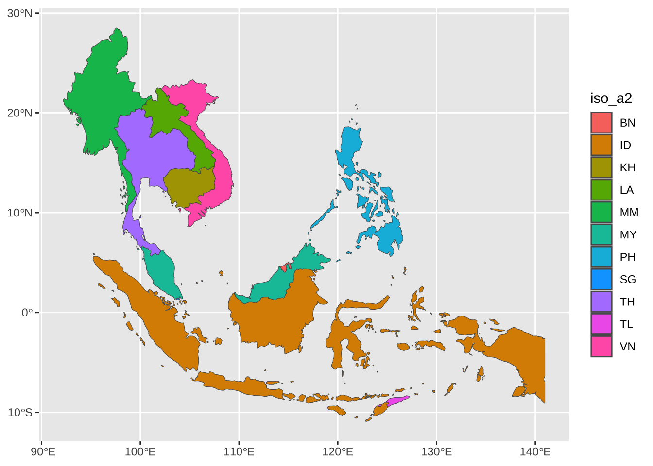

ne_world %>% filter(subregion == "South-Eastern Asia") %>%
  ggplot() +   geom_sf(aes(fill = iso_a2))

ne_world %>% filter(continent == 'Africa') %>%
  ggplot() +   geom_sf(aes(fill = subregion))

C.2.1.3 `type` argument

ne_countries(type = "countries", country = c("Japan", "South Korea", "North Korea", "China", "Taiwan", "Mongolia"), scale = "medium", returnclass = "sf") %>%
  ggplot() + geom_sf(aes(fill = economy))

C.2.2 `ne_states`

Get natural earth world state (admin level 1) polygons

Description: returns state polygons (administrative level 1) for specified countries

C.2.2.1 Usage

ne_states(
  country = NULL,
  geounit = NULL,
  iso_a2 = NULL,
  spdf = NULL,
  returnclass = c("sp", "sf")
)

C.2.3 Arguments

country: a character vector of country names.
geounit: a character vector of geounit names.
iso_a2: a character vector of iso_a2 country codes
spdf: an optional alternative states map
returnclass: ‘sp’ default or ‘sf’ for Simple Features

C.2.4 Value

SpatialPolygons DataFrame or sf

ne_world_admin1 <- ne_states(returnclass = "sf")

glimpse(ne_world_admin1)
#> Rows: 4,596
#> Columns: 122
#> $ featurecla <chr> "Admin-1 states provinces lakes", "Admi…
#> $ scalerank  <int> 3, 6, 2, 6, 3, 4, 4, 3, 4, 3, 4, 3, 3, …
#> $ adm1_code  <chr> "ARG-1309", "URY-8", "IDN-1185", "MYS-1…
#> $ diss_me    <int> 1309, 8, 1185, 1186, 2694, 1936, 1937, …
#> $ iso_3166_2 <chr> "AR-E", "UY-PA", "ID-KI", "MY-12", "CL-…
#> $ wikipedia  <chr> NA, NA, NA, NA, NA, NA, NA, NA, NA, NA,…
#> $ iso_a2     <chr> "AR", "UY", "ID", "MY", "CL", "BO", "BO…
#> $ adm0_sr    <int> 1, 1, 5, 5, 1, 1, 1, 1, 1, 1, 1, 1, 1, …
#> $ name       <chr> "Entre Ríos", "Paysandú", "Kalimantan T…
#> $ name_alt   <chr> "Entre-Rios", NA, "Kaltim", "North Born…
#> $ name_local <chr> NA, NA, NA, NA, NA, NA, NA, NA, NA, NA,…
#> $ type       <chr> "Provincia", "Departamento", "Propinsi"…
#> $ type_en    <chr> "Province", "Department", "Province", "…
#> $ code_local <chr> NA, NA, NA, NA, NA, NA, NA, NA, NA, NA,…
#> $ code_hasc  <chr> "AR.ER", "UY.PA", "ID.KI", "MY.SA", "CL…
#> $ note       <chr> NA, NA, NA, NA, NA, NA, NA, NA, NA, NA,…
#> $ hasc_maybe <chr> NA, NA, NA, NA, NA, NA, NA, NA, "BO.OR|…
#> $ region     <chr> NA, NA, NA, NA, NA, NA, NA, NA, NA, NA,…
#> $ region_cod <chr> NA, NA, NA, NA, NA, NA, NA, NA, NA, NA,…
#> $ provnum_ne <int> 10, 19, 15, 1, 0, 8, 7, 0, 1, 20006, 8,…
#> $ gadm_level <int> 1, 1, 1, 1, 1, 1, 1, 1, 1, 1, 1, 1, 1, …
#> $ check_me   <int> 20, 0, 20, 20, 20, 0, 0, 20, 10, 20, 10…
#> $ datarank   <int> 3, 8, 1, 6, 3, 8, 6, 3, 6, 3, 5, 3, 3, …
#> $ abbrev     <chr> NA, NA, NA, NA, NA, NA, NA, NA, NA, NA,…
#> $ postal     <chr> "ER", "PA", "KI", "SA", NA, "LP", "OR",…
#> $ area_sqkm  <int> 0, 0, 0, 0, 0, 0, 0, 0, 0, 0, 0, 0, 0, …
#> $ sameascity <int> -99, -99, -99, -99, 7, 6, 6, -99, -99, …
#> $ labelrank  <int> 3, 6, 2, 6, 7, 6, 6, 3, 4, 6, 7, 6, 3, …
#> $ name_len   <int> 10, 8, 16, 5, 18, 6, 5, 8, 6, 11, 5, 5,…
#> $ mapcolor9  <int> 3, 2, 6, 3, 5, 2, 2, 5, 2, 5, 4, 3, 3, …
#> $ mapcolor13 <int> 13, 10, 11, 6, 9, 3, 3, 9, 3, 9, 11, 13…
#> $ fips       <chr> "AR08", "UY11", "ID14", "MY16", NA, "BL…
#> $ fips_alt   <chr> NA, NA, NA, NA, NA, NA, NA, NA, "BL05",…
#> $ woe_id     <int> 2344682, 2347650, 2345723, 2346310, 560…
#> $ woe_label  <chr> "Entre Rios, AR, Argentina", "PaysandÃº…
#> $ woe_name   <chr> "Entre Ríos", "Paysandú", "Kalimantan T…
#> $ latitude   <dbl> -32.02750, -32.09330, 1.28915, 5.31115,…
#> $ longitude  <dbl> -59.28240, -57.22400, 116.35400, 117.09…
#> $ sov_a3     <chr> "ARG", "URY", "IDN", "MYS", "CHL", "BOL…
#> $ adm0_a3    <chr> "ARG", "URY", "IDN", "MYS", "CHL", "BOL…
#> $ adm0_label <int> 2, 2, 2, 2, 2, 2, 2, 2, 2, 2, 2, 2, 2, …
#> $ admin      <chr> "Argentina", "Uruguay", "Indonesia", "M…
#> $ geonunit   <chr> "Argentina", "Uruguay", "Indonesia", "M…
#> $ gu_a3      <chr> "ARG", "URY", "IDN", "MYS", "CHL", "BOL…
#> $ gn_id      <int> 3434137, 3441242, 1641897, 1733039, 669…
#> $ gn_name    <chr> "Provincia de Entre Rios", "Departament…
#> $ gns_id     <int> -988655, -908097, -2680740, -2405166, 1…
#> $ gns_name   <chr> "Entre Rios", "Paysandu, Departamento d…
#> $ gn_level   <int> 1, 1, 1, 1, 1, 1, 1, 1, 1, 1, 1, 1, 1, …
#> $ gn_region  <chr> NA, NA, NA, NA, NA, NA, NA, NA, NA, NA,…
#> $ gn_a1_code <chr> "AR.08", "UY.11", "ID.14", "MY.16", "CL…
#> $ region_sub <chr> NA, NA, NA, NA, NA, NA, NA, NA, NA, NA,…
#> $ sub_code   <chr> NA, NA, NA, NA, NA, NA, NA, NA, NA, NA,…
#> $ gns_level  <int> 1, 1, 1, 1, 1, 1, 1, 1, 1, 1, 1, 1, 1, …
#> $ gns_lang   <chr> "khm", "fra", "ind", "fil", "ara", "kor…
#> $ gns_adm1   <chr> "AR08", "UY11", "ID14", "MY16", "CI16",…
#> $ gns_region <chr> NA, NA, NA, NA, NA, NA, NA, NA, NA, NA,…
#> $ min_label  <dbl> 6.0, 8.0, 5.0, 7.0, 6.0, 6.6, 6.6, 6.0,…
#> $ max_label  <dbl> 11.0, 11.0, 10.1, 11.0, 11.0, 11.0, 11.…
#> $ min_zoom   <dbl> 6.0, 8.0, 4.6, 7.0, 6.0, 6.6, 6.6, 6.0,…
#> $ wikidataid <chr> "Q44762", "Q16576", "Q3899", "Q179029",…
#> $ name_ar    <chr> "إنتري ريوس", "إدارة بايساندو", "كالمنت…
#> $ name_bn    <chr> "এন্ত্রে রিও প্রদেশ", "পেসান্ডো বিভাগ", "পূর্…
#> $ name_de    <chr> "Entre Ríos", "Paysandú", "Ostkalimanta…
#> $ name_en    <chr> "Entre Ríos", "Paysandú", "East Kaliman…
#> $ name_es    <chr> "Entre Ríos", "Paysandú", "Kalimantan O…
#> $ name_fr    <chr> "Entre Ríos", "Paysandú", "Kalimantan o…
#> $ name_el    <chr> "Έντρε Ρίος", "Παϊσαντού", "Ανατολικό Κ…
#> $ name_hi    <chr> "एन्ट्रे रियोस", "पयसंदु विभाग", "पूर्व कालिमंत…
#> $ name_hu    <chr> "Entre Ríos", "Paysandú", "Kelet-Kalima…
#> $ name_id    <chr> "Entre Ríos", "Departemen Paysandú", "K…
#> $ name_it    <chr> "Entre Ríos", "dipartimento di Paysandú…
#> $ name_ja    <chr> "エントレ・リオス州", "パイサンドゥ県",…
#> $ name_ko    <chr> "엔트레리오스", "파이산두", "동칼리만탄…
#> $ name_nl    <chr> "Entre Ríos", "Paysandú", "Oost-Kaliman…
#> $ name_pl    <chr> "Entre Ríos", "Paysandú", "Borneo Wscho…
#> $ name_pt    <chr> "Entre Ríos", "Paysandú", "Kalimantan O…
#> $ name_ru    <chr> "Энтре-Риос", "Пайсанду", "Восточный Ка…
#> $ name_sv    <chr> "Entre Ríos", "Paysandú", "Kalimantan T…
#> $ name_tr    <chr> "Entre Ríos eyaleti", "Paysandu Departm…
#> $ name_vi    <chr> "Entre Ríos", "Paysandú", "Đông Kaliman…
#> $ name_zh    <chr> "恩特雷里奥斯省", "派桑杜省", "东加里曼…
#> $ ne_id      <dbl> 1159309789, 1159307733, 1159310009, 115…
#> $ name_he    <chr> "אנטרה ריוס", "פאיסאנדו", "מזרח קלימנטא…
#> $ name_uk    <chr> "Ентре-Ріос", "Пайсанду", "Східний Калі…
#> $ name_ur    <chr> "صوبہ انترے ریوس", "پایساندو محکمہ", "م…
#> $ name_fa    <chr> "ایالت انتره ریوز", "بخش پایساندو", "کا…
#> $ name_zht   <chr> "恩特雷里奥斯省", "派桑杜省", "東加里曼…
#> $ FCLASS_ISO <chr> NA, NA, NA, NA, NA, NA, NA, NA, NA, NA,…
#> $ FCLASS_US  <chr> NA, NA, NA, NA, NA, NA, NA, NA, NA, NA,…
#> $ FCLASS_FR  <chr> NA, NA, NA, NA, NA, NA, NA, NA, NA, NA,…
#> $ FCLASS_RU  <chr> NA, NA, NA, NA, NA, NA, NA, NA, NA, NA,…
#> $ FCLASS_ES  <chr> NA, NA, NA, NA, NA, NA, NA, NA, NA, NA,…
#> $ FCLASS_CN  <chr> NA, NA, NA, NA, NA, NA, NA, NA, NA, NA,…
#> $ FCLASS_TW  <chr> NA, NA, NA, NA, NA, NA, NA, NA, NA, NA,…
#> $ FCLASS_IN  <chr> NA, NA, NA, NA, NA, NA, NA, NA, NA, NA,…
#> $ FCLASS_NP  <chr> NA, NA, NA, NA, NA, NA, NA, NA, NA, NA,…
#> $ FCLASS_PK  <chr> NA, NA, NA, NA, NA, NA, NA, NA, NA, NA,…
#> $ FCLASS_DE  <chr> NA, NA, NA, NA, NA, NA, NA, NA, NA, NA,…
#> $ FCLASS_GB  <chr> NA, NA, NA, NA, NA, NA, NA, NA, NA, NA,…
#> $ FCLASS_BR  <chr> NA, NA, NA, NA, NA, NA, NA, NA, NA, NA,…
#> $ FCLASS_IL  <chr> NA, NA, NA, NA, NA, NA, NA, NA, NA, NA,…
#> $ FCLASS_PS  <chr> NA, NA, NA, NA, NA, NA, NA, NA, NA, NA,…
#> $ FCLASS_SA  <chr> NA, NA, NA, NA, NA, NA, NA, NA, NA, NA,…
#> $ FCLASS_EG  <chr> NA, NA, NA, NA, NA, NA, NA, NA, NA, NA,…
#> $ FCLASS_MA  <chr> NA, NA, NA, NA, NA, NA, NA, NA, NA, NA,…
#> $ FCLASS_PT  <chr> NA, NA, NA, NA, NA, NA, NA, NA, NA, NA,…
#> $ FCLASS_AR  <chr> NA, NA, NA, NA, NA, NA, NA, NA, NA, NA,…
#> $ FCLASS_JP  <chr> NA, NA, NA, NA, NA, NA, NA, NA, NA, NA,…
#> $ FCLASS_KO  <chr> NA, NA, NA, NA, NA, NA, NA, NA, NA, NA,…
#> $ FCLASS_VN  <chr> NA, NA, NA, NA, NA, NA, NA, NA, NA, NA,…
#> $ FCLASS_TR  <chr> NA, NA, NA, NA, NA, NA, NA, NA, NA, NA,…
#> $ FCLASS_ID  <chr> NA, NA, NA, NA, NA, NA, NA, NA, NA, NA,…
#> $ FCLASS_PL  <chr> NA, NA, NA, NA, NA, NA, NA, NA, NA, NA,…
#> $ FCLASS_GR  <chr> NA, NA, NA, NA, NA, NA, NA, NA, NA, NA,…
#> $ FCLASS_IT  <chr> NA, NA, NA, NA, NA, NA, NA, NA, NA, NA,…
#> $ FCLASS_NL  <chr> NA, NA, NA, NA, NA, NA, NA, NA, NA, NA,…
#> $ FCLASS_SE  <chr> NA, NA, NA, NA, NA, NA, NA, NA, NA, NA,…
#> $ FCLASS_BD  <chr> NA, NA, NA, NA, NA, NA, NA, NA, NA, NA,…
#> $ FCLASS_UA  <chr> NA, NA, NA, NA, NA, NA, NA, NA, NA, NA,…
#> $ FCLASS_TLC <chr> NA, NA, NA, NA, NA, NA, NA, NA, NA, NA,…
#> $ geometry   <MULTIPOLYGON [°]> MULTIPOLYGON (((-58.20011 …

ne_world_admin1 %>% as_tibble() %>% 
  filter(iso_a2 != "-1") %>% arrange(admin) %>%
  distinct(iso_a2, admin)
#> # A tibble: 243 × 2
#>    iso_a2 admin              
#>    <chr>  <chr>              
#>  1 AF     Afghanistan        
#>  2 AX     Aland              
#>  3 AL     Albania            
#>  4 DZ     Algeria            
#>  5 AS     American Samoa     
#>  6 AD     Andorra            
#>  7 AO     Angola             
#>  8 AI     Anguilla           
#>  9 AQ     Antarctica         
#> 10 AG     Antigua and Barbuda
#> # ℹ 233 more rows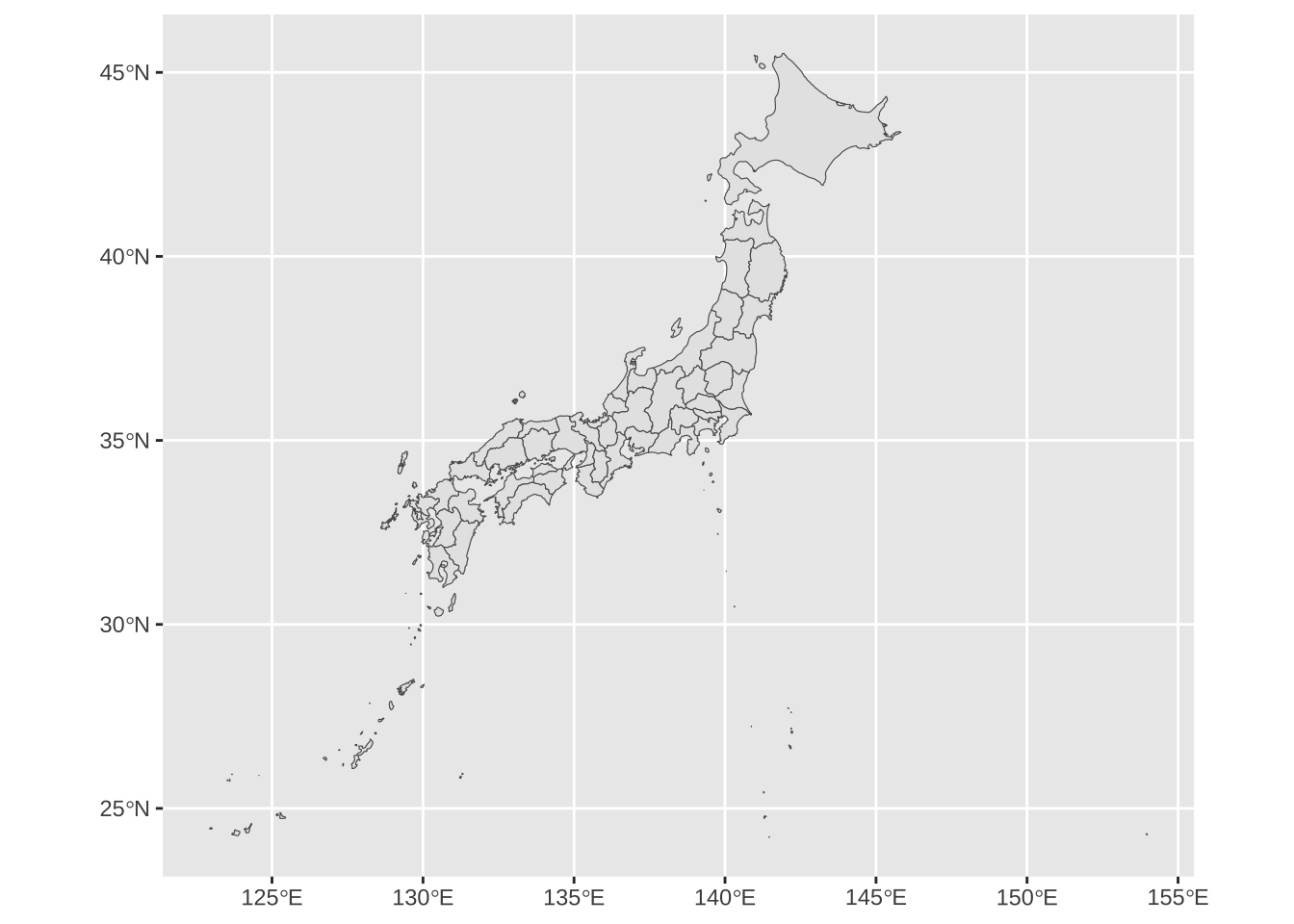

country <- "Japan"
ne_world_admin1 %>% filter(admin == country) %>% 
  ggplot() + geom_sf()

iso2s <- c("IN","PK","BD","LK")
ne_world_admin1 %>% filter(iso_a2 %in% iso2s) %>% 
  ggplot() +   geom_sf(aes(fill = admin))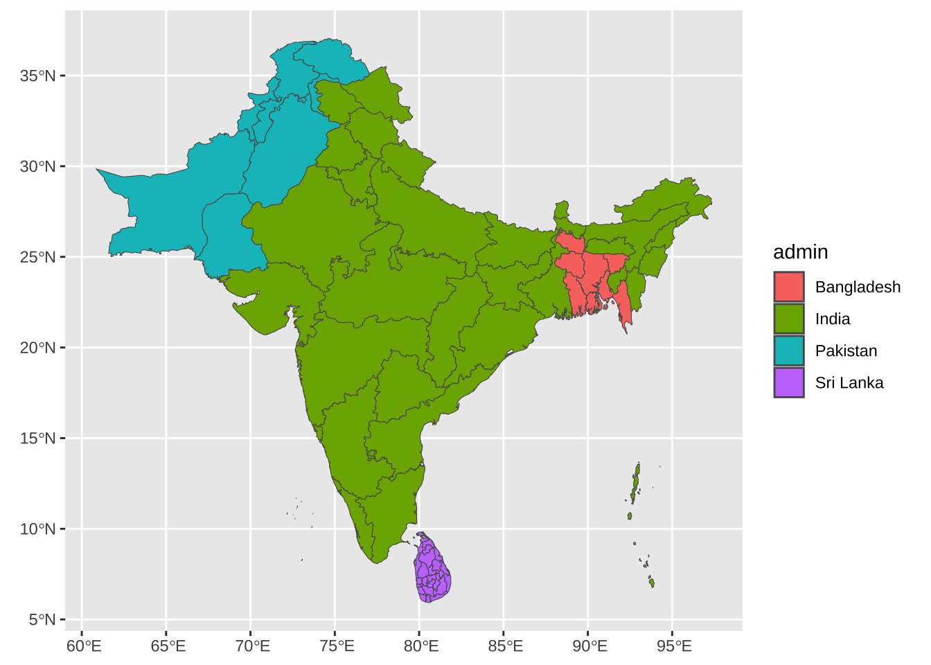

regions <- c("Tohoku")
ne_world_admin1 %>% filter(region %in% regions) %>% 
  ggplot() + geom_sf(aes(fill = name_local))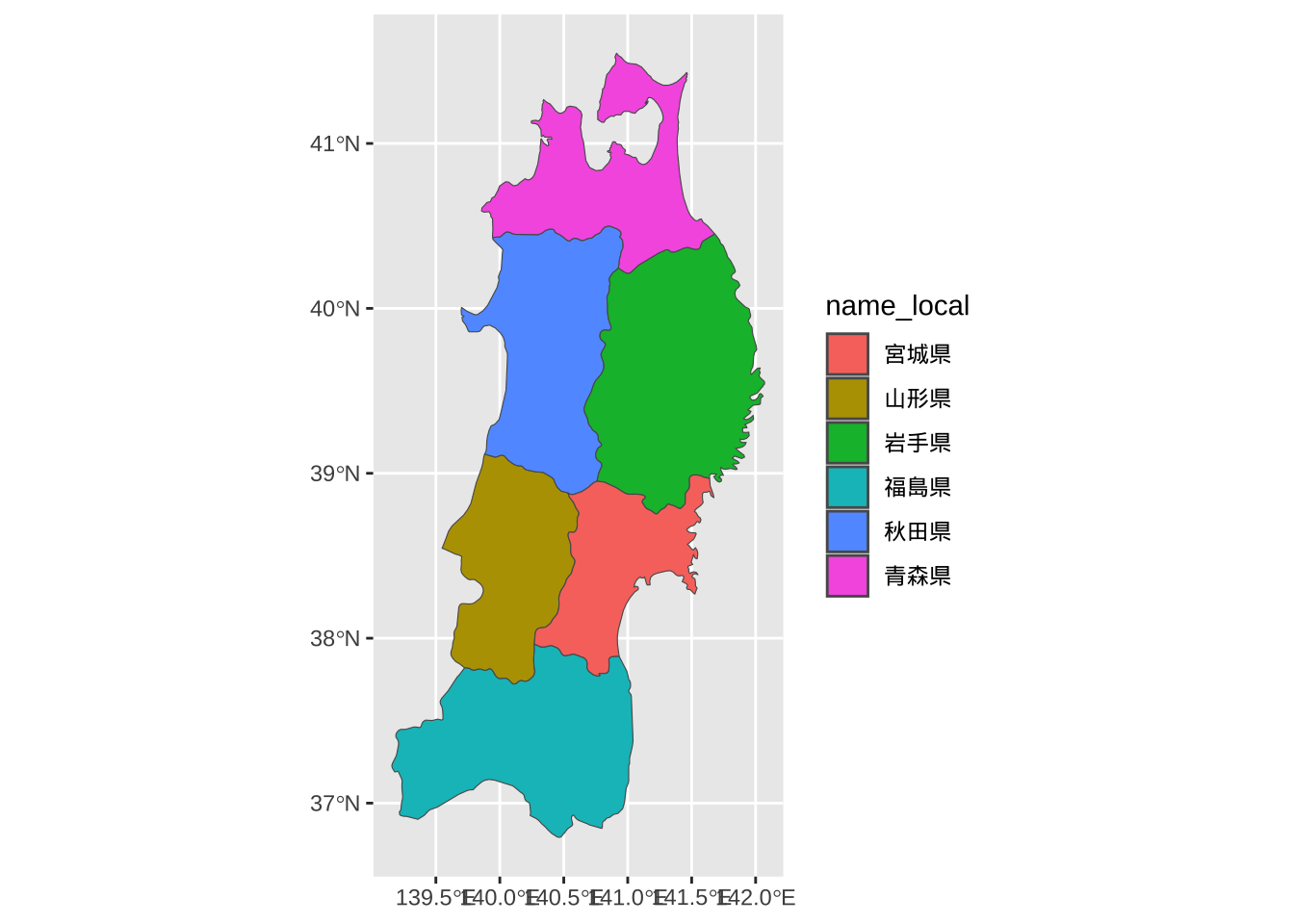

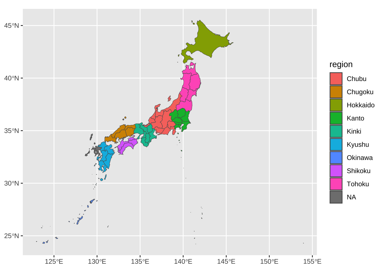
ne_world_admin1 %>% filter(iso_a2 == "JP") %>%
  ggplot() +   geom_sf(aes(fill = region))

ne_world_admin1 %>% as_tibble() %>% filter(admin %in% "Japan") %>% 
  select(name_local, region) %>% filter(is.na(region))
#> # A tibble: 2 × 2
#>   name_local region
#>   <chr>      <chr> 
#> 1 佐賀県     <NA>  
#> 2 長崎県     <NA>

ne_world_admin1 %>% mutate(region = case_when(
  name_local == "佐賀県" ~ "Kyushu",
  name_local == "長崎県" ~ "Kyushu",
  TRUE ~ region)) %>%
  as_tibble() %>% filter(admin %in% "Japan") %>% 
  select(name_local, region) %>% filter(is.na(region))
#> # A tibble: 0 × 2
#> # ℹ 2 variables: name_local <chr>, region <chr>

ne_world_admin1 %>% mutate(region = case_when(
  name_local == "佐賀県" ~ "Kyushu",
  name_local == "長崎県" ~ "Kyushu",
  TRUE ~ region)) %>%
  filter(iso_a2 == "JP") %>%
  ggplot() +   geom_sf(aes(fill = region))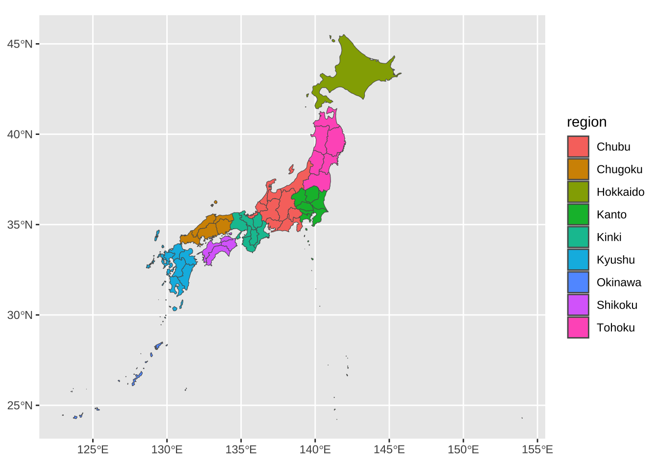

C.3 `geodata` Package

URL: https://gadm.org
geodata: Download Geographic Data
Functions for downloading of geographic data for use in spatial analysis and mapping. The package facilitates access to climate, crops, elevation, land use, soil, species occurrence, accessibility, administrative boundaries and other data.
Package Link: https://CRAN.R-project.org/package=geodata
Manual: https://cran.r-project.org/web/packages/geodata/geodata.pdf

library(geodata)
#> Loading required package: terra
#> terra 1.7.55
#> 
#> Attaching package: 'terra'
#> The following object is masked from 'package:tidyr':
#> 
#>     extract

world(resolution=5, level=0, path = "./data")
#>  class       : SpatVector 
#>  geometry    : polygons 
#>  dimensions  : 231, 2  (geometries, attributes)
#>  extent      : -180, 180, -90, 83.65625  (xmin, xmax, ymin, ymax)
#>  coord. ref. : +proj=longlat +datum=WGS84 +no_defs 
#>  names       : GID_0      NAME_0
#>  type        : <chr>       <chr>
#>  values      :   ABW       Aruba
#>                  AFG Afghanistan
#>                  AGO      Angola

world5 <- readRDS("./data/gadm/gadm36_adm0_r5_pk.rds")
world5 %>% as_tibble() %>% glimpse()
#> Rows: 231
#> Columns: 2
#> $ GID_0  <chr> "ABW", "AFG", "AGO", "ALA", "ALB", "AND", "…
#> $ NAME_0 <chr> "Aruba", "Afghanistan", "Angola", "Åland", …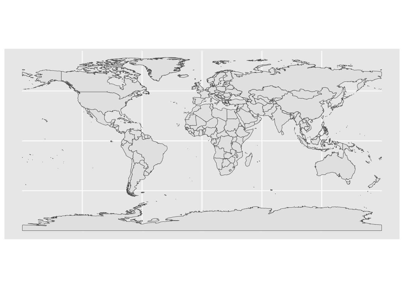

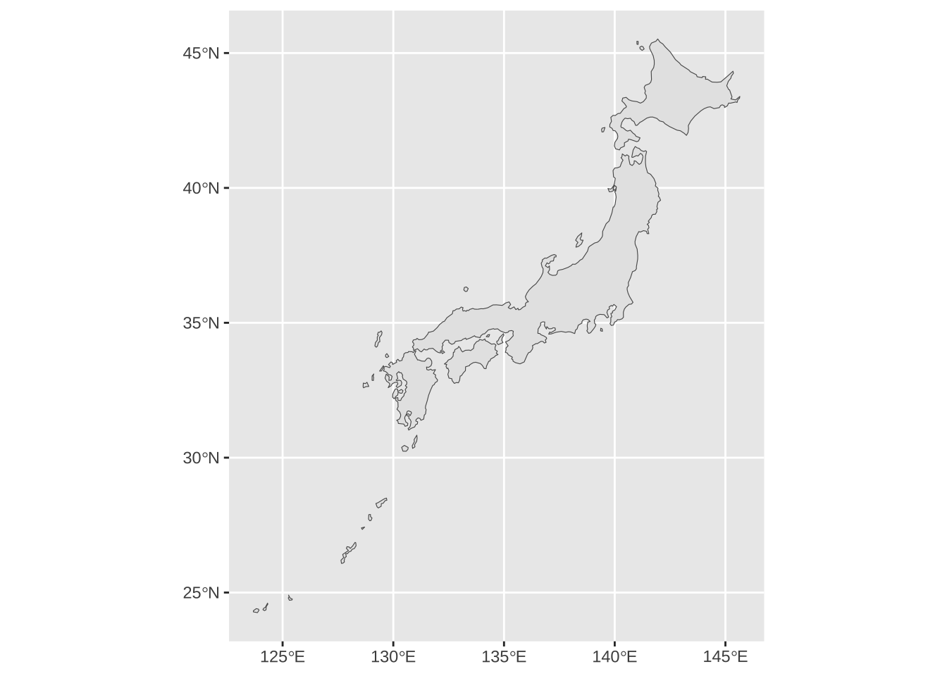
world5 %>% st_as_sf() %>% ggplot() + geom_sf()

world5 %>% 
  st_as_sf() %>% filter(GID_0 == "JPN") %>% 
  ggplot() + geom_sf()

world(resolution=1, level=0, path = "./data") %>%
  st_as_sf() %>% ggplot() + geom_sf()

world(path = "./data") %>%
  st_as_sf() %>% ggplot() + geom_sf()

world(resolution=1, level=0, path = "./data") %>%
  st_as_sf() %>% filter(NAME_0 == "Japan") %>%
  ggplot() + geom_sf()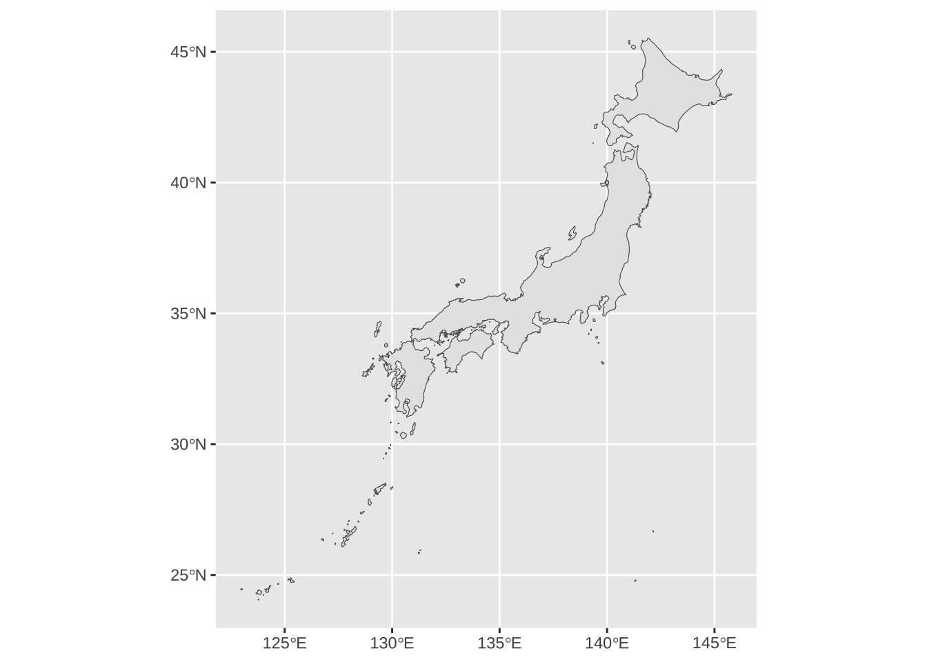

world(resolution=1, level=0, path = "./data") %>%
  st_as_sf() %>% filter(NAME_0 %in% c("India","Pakistan", "Bangladesh" , "Sri Lanka")) %>%
  ggplot() + geom_sf(aes(fill = GID_0))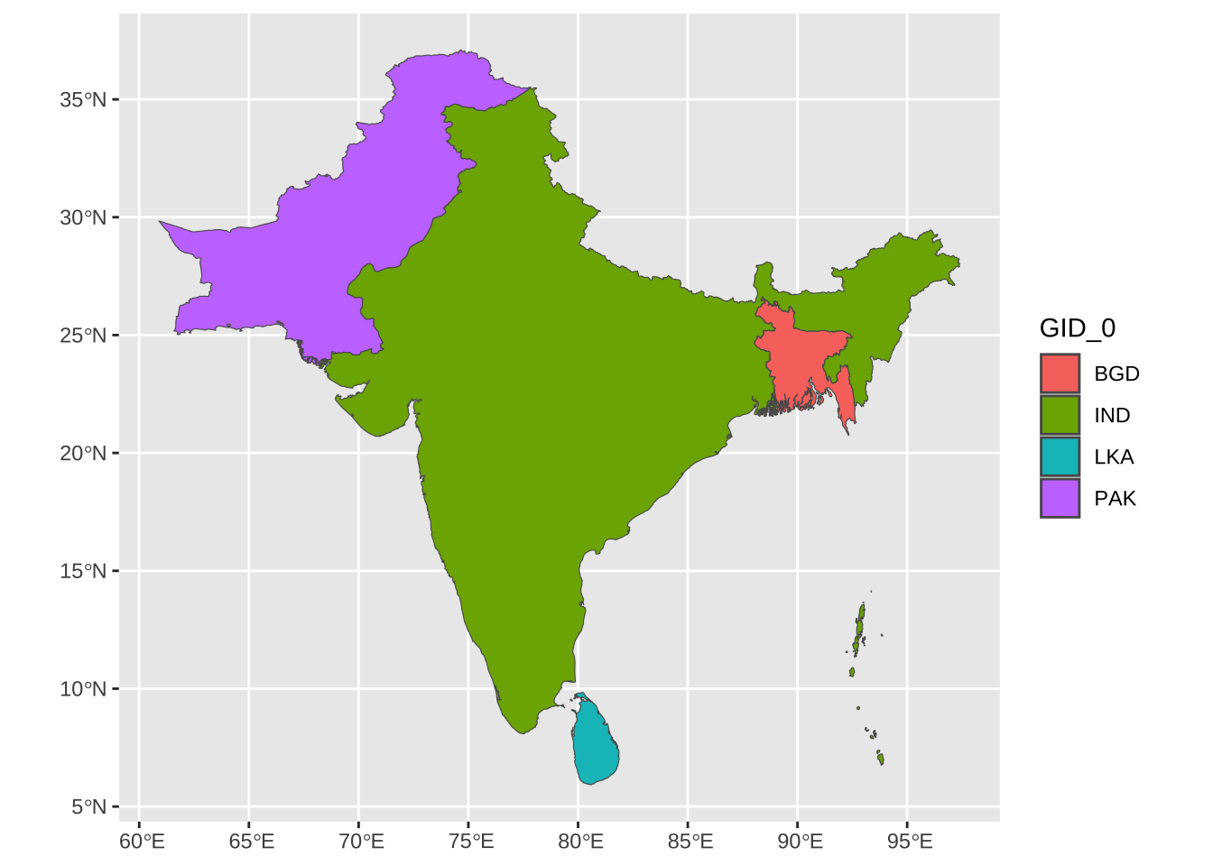

world5_df <- st_as_sf(world5) %>% 
  st_set_crs("+proj=longlat +datum=WGS84") %>% 
  st_transform(., "+proj=robin")

ggplot() +
  geom_sf(data = world5_df)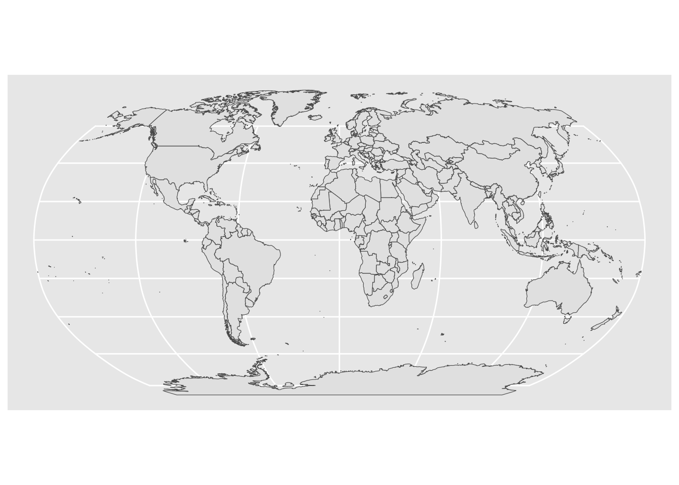

C.3.1 `gadm` Administrative boundaries

Get administrative boundaries for any country in the world. Data are read from files that are down- loaded if necessary.
Usage: gadm(country, level=1, path, version="latest", resolution=1, ...)
Arguments
- country: character. Three-letter ISO code or full country name. If you provide multiple names they are all downloaded and rbind-ed together
- level: numeric. The level of administrative subdivision requested. (starting with 0 for country, then 1 for the first level of subdivision)
- path: character. Path for storing the downloaded data. See geodata_path
- version: character. Either “latest” or GADM version number (can be “3.6”, “4.0” or “4.1”)
- resolution: integer indicating the level of detail. Only for version 4.1. It should be either 1 (high) or 2 (low)

gadm0 <- gadm("JPN", level = 0, path = "./data/")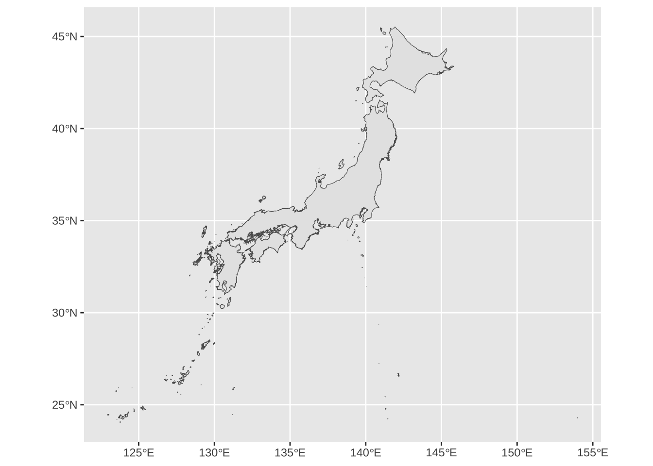

gadm0 %>% st_as_sf() %>% 
  ggplot() + geom_sf()

gadm1 <- gadm("JPN", level = 1, path = "./data/") %>% st_as_sf()
gadm1 %>% glimpse()
#> Rows: 47
#> Columns: 12
#> $ GID_1     <chr> "JPN.1_1", "JPN.2_1", "JPN.3_1", "JPN.4_…
#> $ GID_0     <chr> "JPN", "JPN", "JPN", "JPN", "JPN", "JPN"…
#> $ COUNTRY   <chr> "Japan", "Japan", "Japan", "Japan", "Jap…
#> $ NAME_1    <chr> "Aichi", "Akita", "Aomori", "Chiba", "Eh…
#> $ VARNAME_1 <chr> "Aiti", NA, NA, "Tiba|Tsiba", NA, "Hukui…
#> $ NL_NAME_1 <chr> "愛知県", "秋田県", "青森県", "千葉県", …
#> $ TYPE_1    <chr> "Ken", "Ken", "Ken", "Ken", "Ken", "Ken"…
#> $ ENGTYPE_1 <chr> "Prefecture", "Prefecture", "Prefecture"…
#> $ CC_1      <chr> NA, NA, NA, NA, NA, NA, NA, NA, NA, NA, …
#> $ HASC_1    <chr> "JP.AI", "JP.AK", "JP.AO", "JP.CH", "JP.…
#> $ ISO_1     <chr> "JP-23", "JP-05", "JP-02", "JP-12", "JP-…
#> $ geometry  <GEOMETRY [°]> MULTIPOLYGON (((137.0974 34...,…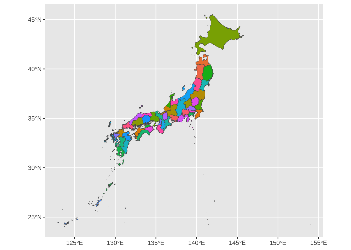

gadm1 %>% 
  ggplot() + geom_sf(aes(fill = NAME_1)) + theme(legend.position = "none")

gadm2 <- gadm("JPN", level = 2, path = "./data/") %>% st_as_sf()
gadm2 %>% glimpse()
#> Rows: 1,811
#> Columns: 14
#> $ GID_2     <chr> "JPN.1.1_1", "JPN.1.2_1", "JPN.1.3_1", "…
#> $ GID_0     <chr> "JPN", "JPN", "JPN", "JPN", "JPN", "JPN"…
#> $ COUNTRY   <chr> "Japan", "Japan", "Japan", "Japan", "Jap…
#> $ GID_1     <chr> "JPN.1_1", "JPN.1_1", "JPN.1_1", "JPN.1_…
#> $ NAME_1    <chr> "Aichi", "Aichi", "Aichi", "Aichi", "Aic…
#> $ NL_NAME_1 <chr> "愛知県", "愛知県", "愛知県", "愛知県", …
#> $ NAME_2    <chr> "Agui", "Aisai", "Anjō", "Chiryū", "Chit…
#> $ VARNAME_2 <chr> NA, NA, NA, NA, NA, NA, NA, NA, NA, NA, …
#> $ NL_NAME_2 <chr> "阿久比町", "愛西市", "安城市", "知立市"…
#> $ TYPE_2    <chr> "Machi", "Shi", "Shi", "Shi", "Shi", "Ma…
#> $ ENGTYPE_2 <chr> "Town", "City", "City", "City", "City", …
#> $ CC_2      <chr> NA, NA, NA, NA, NA, NA, NA, NA, NA, NA, …
#> $ HASC_2    <chr> NA, NA, NA, NA, "JP.AI.CG", NA, NA, "JP.…
#> $ geometry  <GEOMETRY [°]> POLYGON ((136.8802 34.94398...,…

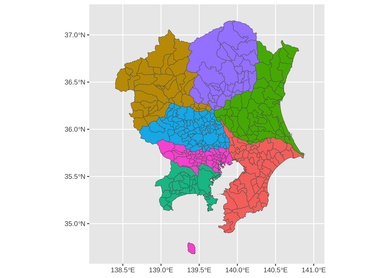
gadm2 %>% filter(NL_NAME_1 %in% c("埼玉県", "群馬県", "栃木県", "茨城県", "千葉県", "神奈川県", "東京都")) %>% 
  ggplot() + geom_sf(aes(fill = NAME_1)) + 
  ylim(34.7,37.2) + xlim(138.2,141) + 
  theme(legend.position = "none")

B Covid 19

D Bookdown