11 Workflow
It is an excellent time to review and sort out the data analysis workflow using R Studio.
library(tidyverse)
#> ── Attaching core tidyverse packages ──── tidyverse 2.0.0 ──
#> ✔ dplyr     1.1.3     ✔ readr     2.1.4
#> ✔ forcats   1.0.0     ✔ stringr   1.5.0
#> ✔ ggplot2   3.4.4     ✔ tibble    3.2.1
#> ✔ lubridate 1.9.3     ✔ tidyr     1.3.0
#> ✔ purrr     1.0.2
#> ── Conflicts ────────────────────── tidyverse_conflicts() ──
#> ✖ dplyr::filter() masks stats::filter()
#> ✖ dplyr::lag()    masks stats::lag()
#> ℹ Use the conflicted package (<http://conflicted.r-lib.org/>) to force all conflicts to become errors
library(WDI)
library(readxl)
11.1 EDA Step 0
- Choose and clarify a topic to study.
- List questions to study
- Find data:
- link to data with a url: universal resource locator in a webpage
- download data in csv, Excel, etc.
Repeat the process during your EDA.
11.2 EDA by R Studio: Step 1
In RStudio,
1.1. Project
- Create a new project: File > New Project; or
- Open a project: File > Open Project, Open Project in New Session, Open Recent Project
- It is easier to find an existing project from: File > Recent Project
- Check there is a file
project_name.Rprojin your project folder (directory)
1.2. data folder (directory) data
- Create a data folder: Press New Folder at the right bottom pane; or
- Confirm the data folder previously created: Press Files at the right bottom pane
- If you follow 1, the data folder exists in your project folder
1.3. Move (or copy) data for the project to the data folder
- If you downloaded the data, it is in your Download folder. Move it to
data. - Check in your RStudio that your data is in
data: Press Files at the right bottom pane and clickdata, the data folder.
11.3 EDA by R Studio: Step 2
2.1. Project Notebook: Memo
-
Create an R Notebook: File > New File > R Notebook
- You can use R Notebook template in Moodle by moving the template (template.Rmd or template.nb.Rmd) file in your project folder or copy and paste the text file into your new R Notebook.
- If you use template.nb.Rmd (R Notebook File), choose Open in Editor.
Add descriptive title.
2.2. Setup Code Chunk
-
Create a code chunk and add packages to use in the project and RUN the code.
- library(tidyverse)
- library(WDI)
- or any other packages
2.3. Choose Source or Visual editor mode, and start editing Project Notebook
Set up Headings such as: About, Data, Analysis and Visualizations, Conclusions
-
Under About or Data, paste url of the sites and/or the data
- eg. World Development Indicator: https://datatopics.worldbank.org/world-development-indicators/)
- eg. Public expenditure on education: https://data.un.org/_Docs/SYB/CSV/SYB65_245_202209_Public% 20expenditure%20on%20education.csv)
2.4. Edit a new file by saving as for a report
- File > Save As…
11.4 EDA by R Studio: Step 3 - Importing Data
Assign a name you can recall easily when you import data. You may need to reload the data with options.
3.1. Use a package:
- WDI, wir, eurostat, etc/
- `wdi_shortname <- WDI(indicator = “indicator’s name”, … )
- Store the data and use it:
write_csv(wdi_shortname, "./data/wdi_shortname.csv") wdi_shortname <- read_csv("./data/wdi_shortname.csv")
3.2. Use readr to read from data, your data folder
df1_shortname <- read_csv("./data/file_name.csv")
3.3. Use readr to read using the url of the data
df2_shortname <- read_csv("url_of_the_data")- Store the data and use it:
write_csv(df2_shortname, "./data/df2_shortname.csv") df2_shortname <- read_csv("./data/df2_shortname.csv")
3.5. Use readxl to read Excel data. Add library(readxl) in the setup and run.
df4 <- read_excel("./data/file_name.xlsx", sheet = 1)
11.5 EDA by R Studio: Step 4 - Data Trasnformation
4.1. Look at the data: suppose df is the data frame
- It is a good option to change into a tibble:
dt <- as_tibble(df) -
head(df),str(df),summary(df),dt,glimpse(dt)
4.2. Look at each variable
- categorical? numerical?
- factor? - forcats
4.3. Variation of each data: suppose x1 is a column name.
df %>% ggplot() + geom_histogram(aes(x1), bins = 30)-
df %>% drop_na(x1): see the rows with a value inx1. If the value is NA, the row is not shown.-
df_wo_na <- df %>% drop_na(x1)if you want to use only the rows without NA inx1
-
4.4. Use dpylr and tidyr to change column names, tidy data, and/or summarize data
-
rename,select,filter,arrange,mutate,pivot_longer(),pivot_wider(),group_byandsummarize
11.6 EDA by R Studio: Step 5 - Visualize Data
5.1. In combination with Stap 4 - data transformation, try various data visualization.
- What type of variation occurs within my variables?
- What type of covariation occurs between my variables?
5.2. Keep a record of what you can observe by the visualization
5.3. Edit the list of questions by adding or polishing
5.4. Select several informative chart and add options
5.5. Look at examples from the textbooks or teaching site to have better visualization
References: Cheat Sheet - ggplot2 ggplot2, ggplot2 book
11.7 EDA by R Studio: Step 6 - Conclusions and Questions for Further Study
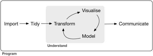
EDA is an iterative cycle that helps you understand what your data says. When you do EDA, you:
Generate questions about your data
Search for answers by visualising, transforming, and/or modeling your data
Use what you learn to refine your questions and/or generate new questions
EDA is an important part of any data analysis. You can use EDA to make discoveries about the world; or you can use EDA to ensure the quality of your data, asking questions about whether the data meets your standards or not.
11.9 Example: WIR2022
df_f8 <- read_excel("./data/WIR2022s.xlsx", sheet = "data-F8")
df_f8
#> # A tibble: 51 × 17
#>     year Germany `Germany (private)` Spain `Spain (private)`
#>    <dbl>   <dbl>               <dbl> <dbl>             <dbl>
#>  1  1970   1.11                 2.30 0.604              4.06
#>  2  1971   1.12                 2.25 0.657              4.53
#>  3  1972   1.11                 2.27 0.624              4.36
#>  4  1973   1.11                 2.23 0.596              4.46
#>  5  1974   1.13                 2.25 0.586              4.64
#>  6  1975   1.12                 2.35 0.602              4.83
#>  7  1976   1.03                 2.34 0.581              4.46
#>  8  1977   1.01                 2.42 0.586              4.10
#>  9  1978   0.990                2.52 0.604              4.10
#> 10  1979   0.989                2.55 0.621              4.20
#> # ℹ 41 more rows
#> # ℹ 12 more variables: France <dbl>,
#> #   `France (private)` <dbl>, UK <dbl>,
#> #   `UK (private)` <dbl>, Japan <dbl>,
#> #   `Japan (private)` <dbl>, Norway <dbl>,
#> #   `Norway (private)` <dbl>, USA <dbl>,
#> #   `USA (private)` <dbl>, gwealAVGRICH <dbl>, …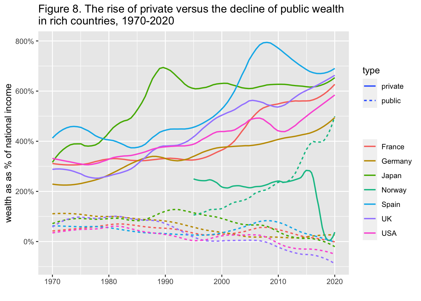
11.10 The Week Five Assignment (in Moodle)
tidyr and WIR2022
- Create an R Notebook of a Data Analysis containing the following and submit the rendered HTML file (eg.
a3_123456.nb.htmlby replacing 123456 with your ID)- create an R Notebook using the R Notebook Template in Moodle, save as
a3_123456.Rmd, - write your name and ID and the contents,
- run each code block,
- preview to create
a3_123456.nb.html, - submit
a3_123456.nb.htmlto Moodle.
- create an R Notebook using the R Notebook Template in Moodle, save as
-
Choose a data with at least two categorical variables and at least two numerical variables.
- Information of the data: Name, Indicator, Description, Source, etc.
- Explain why you chose the indicator
- List questions you want to study
-
Explore the data using visualization using
ggplot2- Create various charts
- Create at least one chart with at least two categocial variables and at least one numerical variable.
- Create at least one chart with at least two numerical variables and at least one categorical variable.
Observations based on your data visualization, and difficulties and questions encountered if any.
Due: 2023-01-23 23:59:00. Submit your R Notebook file in Moodle (The Fourth Assignment). Due on Monday!