5 dplyr
The
dplyris a package to transform data. It can combine data as well. We will treat the second feature late in Chapter ??. The packagedplyris a part of thetidyversepackages, and you do not need to install it separately.
library(tidyverse)
#> ── Attaching core tidyverse packages ──── tidyverse 2.0.0 ──
#> ✔ dplyr     1.1.3     ✔ readr     2.1.4
#> ✔ forcats   1.0.0     ✔ stringr   1.5.0
#> ✔ ggplot2   3.4.4     ✔ tibble    3.2.1
#> ✔ lubridate 1.9.3     ✔ tidyr     1.3.0
#> ✔ purrr     1.0.2
#> ── Conflicts ────────────────────── tidyverse_conflicts() ──
#> ✖ dplyr::filter() masks stats::filter()
#> ✖ dplyr::lag()    masks stats::lag()
#> ℹ Use the conflicted package (<http://conflicted.r-lib.org/>) to force all conflicts to become errors
5.1 dplyr Overview
dplyr is a grammar of data manipulation, providing a consistent set of verbs that help you solve the most common data manipulation challenges:
-
select()picks variables based on their names. -
filter()picks cases based on their values. -
mutate()adds new variables that are functions of existing variables -
summarise()reduces multiple values down to a single summary. -
arrange()changes the ordering of the rows. -
group_by()takes an existing tbl and converts it into a grouped tbl.
You can learn more about them in vignette(“dplyr”). As well as these single-table verbs, dplyr also provides a variety of two-table verbs, which you can learn about in vignette(“two-table”).
If you are new to dplyr, the best place to start is the data transformation chapter in R for data science.
5.2 select: Subset columns using their names and types
| Helper Function | Use | Example |
|---|---|---|
| - | Columns except | select(babynames, -prop) |
| : | Columns between (inclusive) | select(babynames, year:n) |
| contains() | Columns that contains a string | select(babynames, contains(“n”)) |
| ends_with() | Columns that ends with a string | select(babynames, ends_with(“n”)) |
| matches() | Columns that matches a regex | select(babynames, matches(“n”)) |
| num_range() | Columns with a numerical suffix in the range | Not applicable with babynames |
| one_of() | Columns whose name appear in the given set | select(babynames, one_of(c(“sex”, “gender”))) |
| starts_with() | Columns that starts with a string | select(babynames, starts_with(“n”)) |
5.3 filter: Subset rows using column values
| Logical operator | tests | Example |
|---|---|---|
| > | Is x greater than y? | x > y |
| >= | Is x greater than or equal to y? | x >= y |
| < | Is x less than y? | x < y |
| <= | Is x less than or equal to y? | x <= y |
| == | Is x equal to y? | x == y |
| != | Is x not equal to y? | x != y |
| is.na() | Is x an NA? | is.na(x) |
| !is.na() | Is x not an NA? | !is.na(x) |
5.4 arrange and Pipe %>%
-
arrange()orders the rows of a data frame by the values of selected columns.
Unlike other dplyr verbs, arrange() largely ignores grouping; you need to explicitly mention grouping variables (`or use .by_group = TRUE) in order to group by them, and functions of variables are evaluated once per data frame, not once per group.
-
pipesin R for Data Science.
5.5 mutate
Create, modify, and delete columns
-
Useful mutate functions
+, -, log(), etc., for their usual mathematical meanings
lead(), lag()
dense_rank(), min_rank(), percent_rank(), row_number(), cume_dist(), ntile()
cumsum(), cummean(), cummin(), cummax(), cumany(), cumall()
na_if(), coalesce()###
group_by()andsummarise()
5.6 group_by
5.7 summarise or summarize
5.7.0.1 Summary functions
So far our summarise() examples have relied on sum(), max(), and mean(). But you can use any function in summarise() so long as it meets one criteria: the function must take a vector of values as input and return a single value as output. Functions that do this are known as summary functions and they are common in the field of descriptive statistics. Some of the most useful summary functions include:
- Measures of location - mean(x), median(x), quantile(x, 0.25), min(x), and max(x)
- Measures of spread - sd(x), var(x), IQR(x), and mad(x)
- Measures of position - first(x), nth(x, 2), and last(x)
- Counts - n_distinct(x) and n(), which takes no arguments, and returns the size of the current group or data frame.
- Counts and proportions of logical values - sum(!is.na(x)), which counts the number of TRUEs returned by a logical test; mean(y == 0), which returns the proportion of TRUEs returned by a logical test.
- if_else(), recode(), case_when()
5.8 Learn dplyr by Examples
5.8.1 Data iris
head(iris)
#>   Sepal.Length Sepal.Width Petal.Length Petal.Width Species
#> 1          5.1         3.5          1.4         0.2  setosa
#> 2          4.9         3.0          1.4         0.2  setosa
#> 3          4.7         3.2          1.3         0.2  setosa
#> 4          4.6         3.1          1.5         0.2  setosa
#> 5          5.0         3.6          1.4         0.2  setosa
#> 6          5.4         3.9          1.7         0.4  setosa
summary(iris)
#>   Sepal.Length    Sepal.Width     Petal.Length
#>  Min.   :4.300   Min.   :2.000   Min.   :1.000
#>  1st Qu.:5.100   1st Qu.:2.800   1st Qu.:1.600
#>  Median :5.800   Median :3.000   Median :4.350
#>  Mean   :5.843   Mean   :3.057   Mean   :3.758
#>  3rd Qu.:6.400   3rd Qu.:3.300   3rd Qu.:5.100
#>  Max.   :7.900   Max.   :4.400   Max.   :6.900
#>   Petal.Width          Species
#>  Min.   :0.100   setosa    :50
#>  1st Qu.:0.300   versicolor:50
#>  Median :1.300   virginica :50
#>  Mean   :1.199
#>  3rd Qu.:1.800
#>  Max.   :2.500
5.8.2 select 1 - columns 1, 2, 5
head(select(iris, c(1,2,5)))
#>   Sepal.Length Sepal.Width Species
#> 1          5.1         3.5  setosa
#> 2          4.9         3.0  setosa
#> 3          4.7         3.2  setosa
#> 4          4.6         3.1  setosa
#> 5          5.0         3.6  setosa
#> 6          5.4         3.9  setosa
You can select the first, the second and the fifth columns. If you want to use it, then assign a new name.
head(iris)
#>   Sepal.Length Sepal.Width Petal.Length Petal.Width Species
#> 1          5.1         3.5          1.4         0.2  setosa
#> 2          4.9         3.0          1.4         0.2  setosa
#> 3          4.7         3.2          1.3         0.2  setosa
#> 4          4.6         3.1          1.5         0.2  setosa
#> 5          5.0         3.6          1.4         0.2  setosa
#> 6          5.4         3.9          1.7         0.4  setosa
5.8.3 select 1 using pipe
In the previous example, we used head(select(iris, c(1,2,5))), head comes first because we apply head to the result of select(iris, c(1,2,5)). In order to apply functions in a sequencial order, we can use pipe command. You can get the same result by the following.
iris %>% select(c(1,2,5)) %>% head()
#>   Sepal.Length Sepal.Width Species
#> 1          5.1         3.5  setosa
#> 2          4.9         3.0  setosa
#> 3          4.7         3.2  setosa
#> 4          4.6         3.1  setosa
#> 5          5.0         3.6  setosa
#> 6          5.4         3.9  setosa
All tidyverse functions are designed so that the first argument, i.e., the entry, is the data. So using pipe, iris is assumed to be the first entry of the select function, and select(iris, c(1,2,5)) is the first entry of the head function.
In the following, we use pipes.
5.8.7 filter - by names
filter(iris, Species == "virginica") %>% head()
#>   Sepal.Length Sepal.Width Petal.Length Petal.Width
#> 1          6.3         3.3          6.0         2.5
#> 2          5.8         2.7          5.1         1.9
#> 3          7.1         3.0          5.9         2.1
#> 4          6.3         2.9          5.6         1.8
#> 5          6.5         3.0          5.8         2.2
#> 6          7.6         3.0          6.6         2.1
#>     Species
#> 1 virginica
#> 2 virginica
#> 3 virginica
#> 4 virginica
#> 5 virginica
#> 6 virginica
5.8.9 mutate - rank
iris %>% mutate(sl_rank = min_rank(Sepal.Length)) %>%
  arrange(sl_rank) %>% head()
#>   Sepal.Length Sepal.Width Petal.Length Petal.Width Species
#> 1          4.3         3.0          1.1         0.1  setosa
#> 2          4.4         2.9          1.4         0.2  setosa
#> 3          4.4         3.0          1.3         0.2  setosa
#> 4          4.4         3.2          1.3         0.2  setosa
#> 5          4.5         2.3          1.3         0.3  setosa
#> 6          4.6         3.1          1.5         0.2  setosa
#>   sl_rank
#> 1       1
#> 2       2
#> 3       2
#> 4       2
#> 5       5
#> 6       6
Insert a line break after the pipe command, not before.
5.8.10 group_by and summarize
iris %>%
  group_by(Species) %>%
  summarize(sl = mean(Sepal.Length), sw = mean(Sepal.Width),
  pl = mean(Petal.Length), pw = mean(Petal.Width))
#> # A tibble: 3 × 5
#>   Species       sl    sw    pl    pw
#>   <fct>      <dbl> <dbl> <dbl> <dbl>
#> 1 setosa      5.01  3.43  1.46 0.246
#> 2 versicolor  5.94  2.77  4.26 1.33
#> 3 virginica 6.59 2.97 5.55 2.03- mean:
mean()ormean(x, na.rm = TRUE)- arithmetic mean (average) - median:
median()ormedian(x, na.rm = TRUE)- mid value
For more examples see
5.9 References of dplyr
- Textbook: R for Data Science, Part II Explore
5.9.1 RStudio Primers: See References in Moodle at the bottom
- Work with Data – r4ds: Wrangle, I
5.10 Learn dplyr by Examples II - gapminder
5.10.1 ggplot2 Overview
ggplot2 is a system for declaratively creating graphics, based on The Grammar of Graphics. You provide the data, tell ggplot2 how to map variables to aesthetics, what graphical primitives to use, and it takes care of the details.
Examples
ggplot(data = mpg) +
  geom_point(mapping = aes(x = displ, y = hwy))
ggplot(data = mpg) +
geom_boxplot(mapping = aes(x = class, y = hwy))Template
ggplot(data = <DATA>) +
  <GEOM_FUNCTION>(mapping = aes(<MAPPINGS>))
5.10.1.1 Gapminder and R Package gapminder
Gapminder was founded by Ola Rosling, Anna Rosling Rönnlund, and Hans Rosling
-
Gapminder: https://www.gapminder.org
- Test on Top: You are probably wrong about - upgrade your worldview
- Bubble Chart: https://www.gapminder.org/tools/#$chart-type=bubbles&url=v1
- Dallar Street: https://www.gapminder.org/tools/#$chart-type=bubbles&url=v1
- Data: https://www.gapminder.org/data/
-
R Package gapminder by Jennifer Bryan
-
Package Help
?gapminderorgapminderin the search window of Help- The main data frame gapminder has 1704 rows and 6 variables:
- country: factor with 142 levels
- continent: factor with 5 levels
- year: ranges from 1952 to 2007 in increments of 5 years
- lifeExp: life expectancy at birth, in years
- pop: population
- gdpPercap: GDP per capita (US$, inflation-adjusted)
- The main data frame gapminder has 1704 rows and 6 variables:
5.10.1.2 R Package gapminder data
We will use a tidyverse function slice replacing head. Check slice in the search window under the Help tab on the bottom right pane.
df <- gapminder
df %>% slice(1:10)
#> # A tibble: 10 × 6
#>    country     continent  year lifeExp      pop gdpPercap
#>    <fct>       <fct>     <int>   <dbl>    <int>     <dbl>
#>  1 Afghanistan Asia       1952    28.8  8425333      779.
#>  2 Afghanistan Asia       1957    30.3  9240934      821.
#>  3 Afghanistan Asia       1962    32.0 10267083      853.
#>  4 Afghanistan Asia       1967    34.0 11537966      836.
#>  5 Afghanistan Asia       1972    36.1 13079460      740.
#>  6 Afghanistan Asia       1977    38.4 14880372      786.
#>  7 Afghanistan Asia       1982    39.9 12881816      978.
#>  8 Afghanistan Asia       1987    40.8 13867957      852.
#>  9 Afghanistan Asia       1992    41.7 16317921      649.
#> 10 Afghanistan Asia       1997    41.8 22227415      635.
glimpse(df)
#> Rows: 1,704
#> Columns: 6
#> $ country   <fct> "Afghanistan", "Afghanistan", "Afghanist…
#> $ continent <fct> Asia, Asia, Asia, Asia, Asia, Asia, Asia…
#> $ year      <int> 1952, 1957, 1962, 1967, 1972, 1977, 1982…
#> $ lifeExp   <dbl> 28.801, 30.332, 31.997, 34.020, 36.088, …
#> $ pop       <int> 8425333, 9240934, 10267083, 11537966, 13…
#> $ gdpPercap <dbl> 779.4453, 820.8530, 853.1007, 836.1971, …
summary(df)
#>         country        continent        year
#>  Afghanistan:  12   Africa  :624   Min.   :1952
#>  Albania    :  12   Americas:300   1st Qu.:1966
#>  Algeria    :  12   Asia    :396   Median :1980
#>  Angola     :  12   Europe  :360   Mean   :1980
#>  Argentina  :  12   Oceania : 24   3rd Qu.:1993
#>  Australia  :  12                  Max.   :2007
#>  (Other)    :1632
#>     lifeExp           pop              gdpPercap
#>  Min.   :23.60   Min.   :6.001e+04   Min.   :   241.2
#>  1st Qu.:48.20   1st Qu.:2.794e+06   1st Qu.:  1202.1
#>  Median :60.71   Median :7.024e+06   Median :  3531.8
#>  Mean   :59.47   Mean   :2.960e+07   Mean   :  7215.3
#>  3rd Qu.:70.85   3rd Qu.:1.959e+07   3rd Qu.:  9325.5
#>  Max.   :82.60   Max.   :1.319e+09   Max.   :113523.1
#>
5.10.1.3 Tidyverse::ggplot
5.10.1.3.1 First Try - with failures
You will encounter similar failures. We list three of them.
ggplot(df, aes(x = year, y = lifeExp)) + geom_point()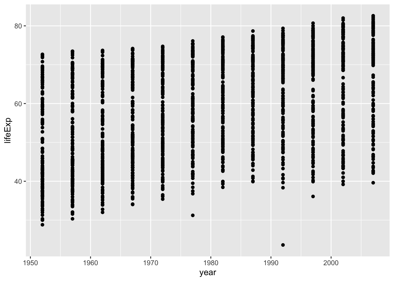
There are lots of data in each year: 1952, 1957, 1962, 1967, 1972, 1977, 1982, 1987, 1992, 1997, …. Can you tell how many years are in the data? The following command shows different years in the data.
unique(df$year)
#>  [1] 1952 1957 1962 1967 1972 1977 1982 1987 1992 1997 2002
#> [12] 2007
You can guess it from the data summary above. Can you imagine how many countries are in the data? 142? Anyhow, too many points are on each year.
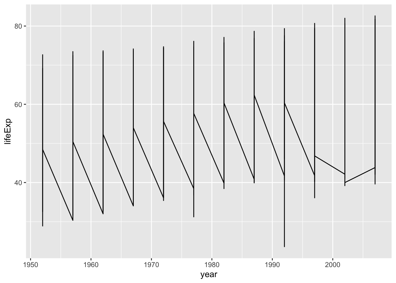
Now, you can guess the reason why you had this output. This is often called a saw-tooth.
ggplot(df, aes(x = year, y = lifeExp)) + geom_boxplot()
#> Warning: Continuous x aesthetic
#> ℹ did you forget `aes(group = ...)`?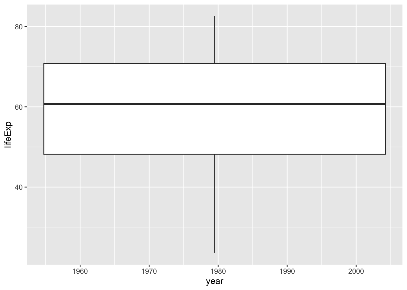
Can you see what the problem is? The year is a numerical variable in integer.
The following looks better.
ggplot(df, aes(y = lifeExp, group = year)) + geom_boxplot()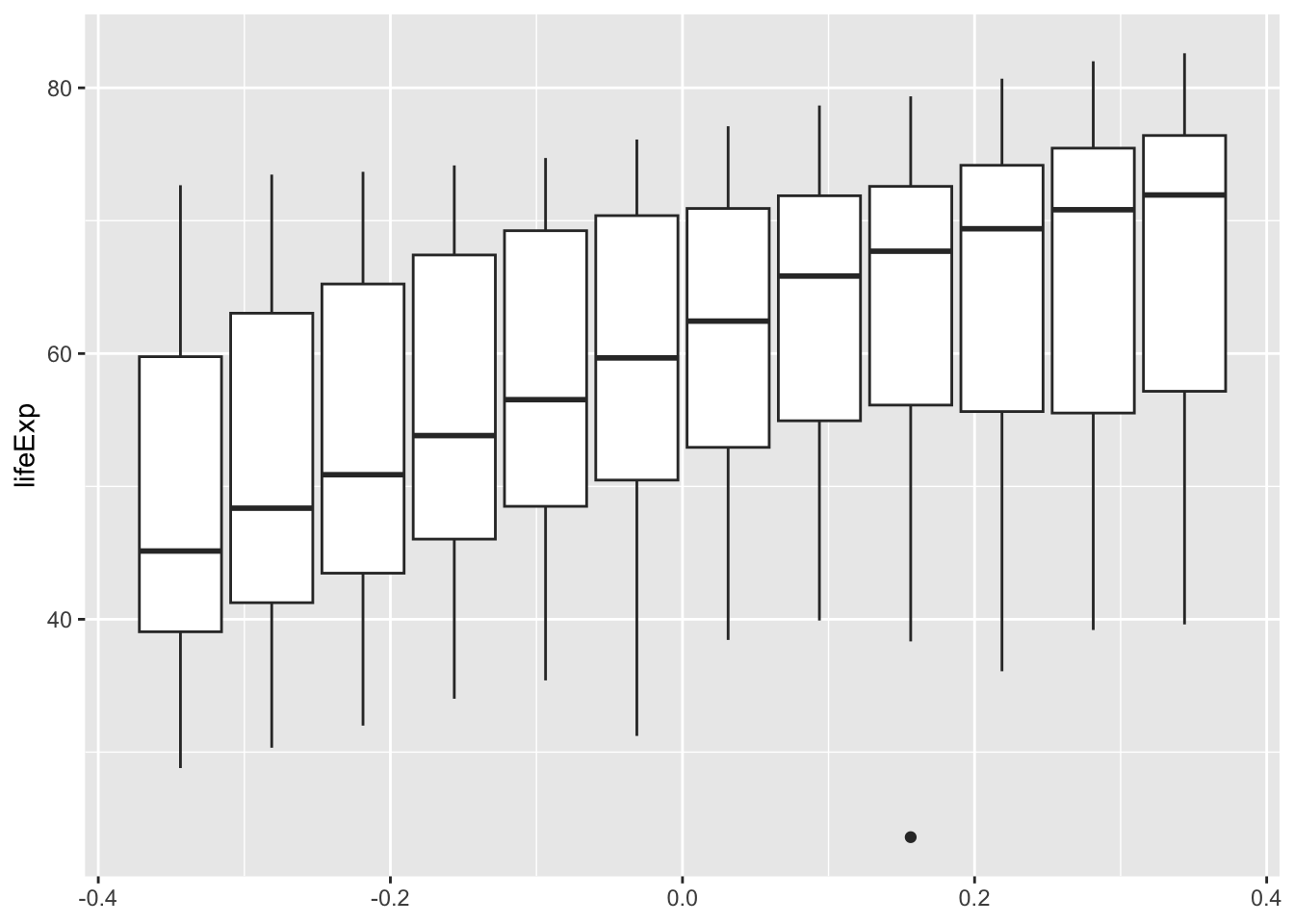
5.10.1.3.2 Box Plot
ggplot(df, aes(x = as_factor(year), y = lifeExp)) + geom_boxplot()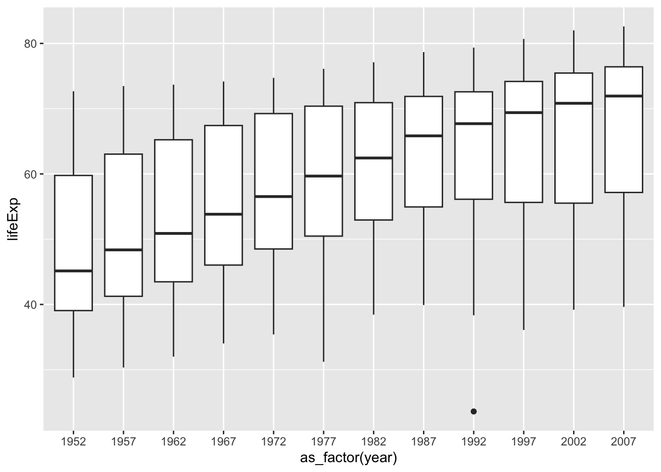
We will study data visualization in Chapter 8.
5.10.1.4 Applications of dplyr
Let us apply dplyr to manipulate data to visualize the data.
5.10.1.4.1 filter
By filter you can obtain the the data of one country.
filter(country == "Afghanistan")
Note that we need two equal symbols, and quotation marks must surround the country name.
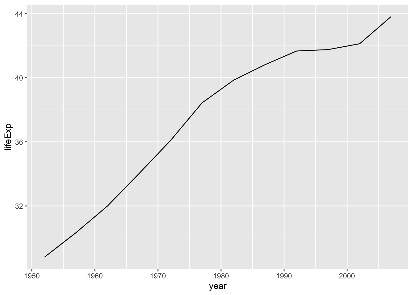
Looks good. From the data you observe, the life expectancy at birth in 1952 was below 30, and it was still below 44 in 2007.
Let us compare Afghanistan with Japan. When you choose more than one country, we use the following format: country %in% c("Afghanistan", "Japan").
df %>% filter(country %in% c("Afghanistan", "Japan")) %>%
  ggplot(aes(x = year, y = lifeExp, color = country)) + geom_line()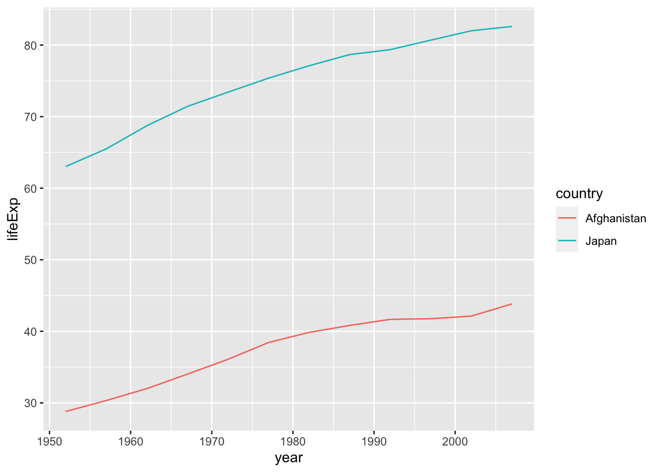
What do you observe from this chart?
The code unique(df$country) does the same as the one below. First, choose distinct elements in the column country by distinct(country) and get the column as a vector by pull.
df %>% distinct(country) %>% pull()
#>   [1] Afghanistan              Albania
#>   [3] Algeria                  Angola
#>   [5] Argentina                Australia
#>   [7] Austria                  Bahrain
#>   [9] Bangladesh               Belgium
#>  [11] Benin                    Bolivia
#>  [13] Bosnia and Herzegovina   Botswana
#>  [15] Brazil                   Bulgaria
#>  [17] Burkina Faso             Burundi
#>  [19] Cambodia                 Cameroon
#>  [21] Canada                   Central African Republic
#>  [23] Chad                     Chile
#>  [25] China                    Colombia
#>  [27] Comoros                  Congo, Dem. Rep.
#>  [29] Congo, Rep.              Costa Rica
#>  [31] Cote d'Ivoire            Croatia
#>  [33] Cuba                     Czech Republic
#>  [35] Denmark                  Djibouti
#>  [37] Dominican Republic       Ecuador
#>  [39] Egypt                    El Salvador
#>  [41] Equatorial Guinea        Eritrea
#>  [43] Ethiopia                 Finland
#>  [45] France                   Gabon
#>  [47] Gambia                   Germany
#>  [49] Ghana                    Greece
#>  [51] Guatemala                Guinea
#>  [53] Guinea-Bissau            Haiti
#>  [55] Honduras                 Hong Kong, China
#>  [57] Hungary                  Iceland
#>  [59] India                    Indonesia
#>  [61] Iran                     Iraq
#>  [63] Ireland                  Israel
#>  [65] Italy                    Jamaica
#>  [67] Japan                    Jordan
#>  [69] Kenya                    Korea, Dem. Rep.
#>  [71] Korea, Rep.              Kuwait
#>  [73] Lebanon                  Lesotho
#>  [75] Liberia                  Libya
#>  [77] Madagascar               Malawi
#>  [79] Malaysia                 Mali
#>  [81] Mauritania               Mauritius
#>  [83] Mexico                   Mongolia
#>  [85] Montenegro               Morocco
#>  [87] Mozambique               Myanmar
#>  [89] Namibia                  Nepal
#>  [91] Netherlands              New Zealand
#>  [93] Nicaragua                Niger
#>  [95] Nigeria                  Norway
#>  [97] Oman                     Pakistan
#>  [99] Panama                   Paraguay
#> [101] Peru                     Philippines
#> [103] Poland                   Portugal
#> [105] Puerto Rico              Reunion
#> [107] Romania                  Rwanda
#> [109] Sao Tome and Principe    Saudi Arabia
#> [111] Senegal                  Serbia
#> [113] Sierra Leone             Singapore
#> [115] Slovak Republic          Slovenia
#> [117] Somalia                  South Africa
#> [119] Spain                    Sri Lanka
#> [121] Sudan                    Swaziland
#> [123] Sweden                   Switzerland
#> [125] Syria                    Taiwan
#> [127] Tanzania                 Thailand
#> [129] Togo                     Trinidad and Tobago
#> [131] Tunisia                  Turkey
#> [133] Uganda                   United Kingdom
#> [135] United States            Uruguay
#> [137] Venezuela                Vietnam
#> [139] West Bank and Gaza       Yemen, Rep.
#> [141] Zambia                   Zimbabwe
#> 142 Levels: Afghanistan Albania Algeria Angola ... Zimbabwe
As we have guessed, there are 142 countries in this data.
Let us choose BRICs countries in the data.
df %>% filter(country %in% c("Brazil", "Russia", "India", "China")) %>%
  ggplot(aes(x = year, y = lifeExp, color = country)) + geom_line()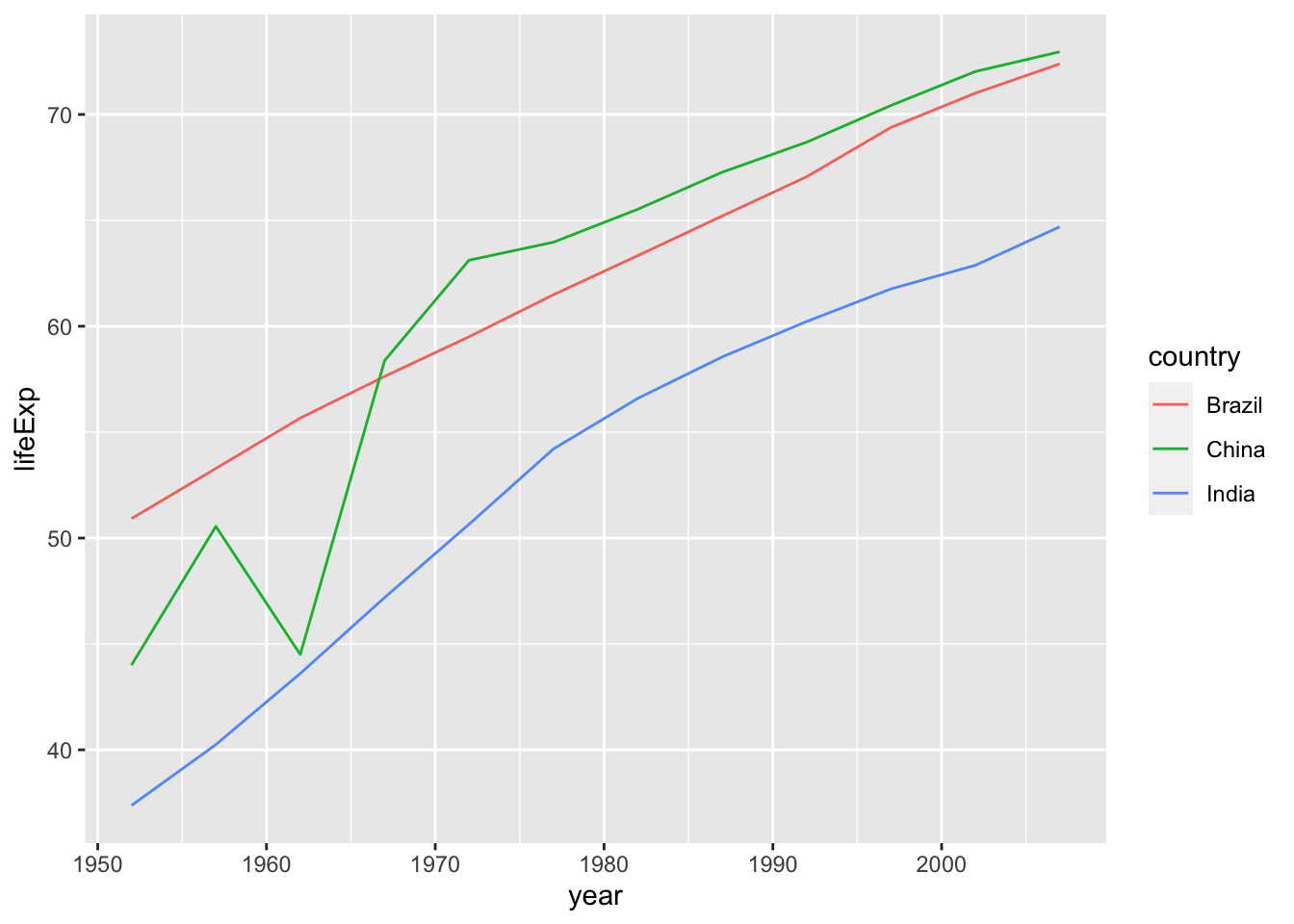
Russia data is missing. Can you find it in the list of countries? It can be a problem of gapminder data. Can you think of the reason why Russia is not in?
5.10.2 Exercises
- Change
lifeExptopopandgdpPercapand do the same. - Choose ASEAN countries and do the similar investigations.
Brunei, Cambodia, Indonesia, Laos, Malaysia, Myanmar, Philippines, Singapore.
How many of these countries are on the list?
- Choose several countries by yourself and do the similar investigations.
5.10.3 group_by and summarize
Let us use the variable continent and summarize the data. Can you tell how many continents are listed in the data? Yes, there are five. Can you tell how many countries are in each continent on the data?
df_lifeExp <- df %>% group_by(continent, year) %>%
  summarize(mean_lifeExp = mean(lifeExp), median_lifeExp = median(lifeExp), max_lifeExp = max(lifeExp), min_lifeExp = min(lifeExp), .groups = "keep")
Don’t get scared. We will learn little by little.
df_lifeExp %>% slice(1:10)
#> # A tibble: 60 × 6
#> # Groups:   continent, year [60]
#>    continent  year mean_lifeExp median_lifeExp max_lifeExp
#>    <fct>     <int>        <dbl>          <dbl>       <dbl>
#>  1 Africa     1952         39.1           38.8        52.7
#>  2 Africa     1957         41.3           40.6        58.1
#>  3 Africa     1962         43.3           42.6        60.2
#>  4 Africa     1967         45.3           44.7        61.6
#>  5 Africa     1972         47.5           47.0        64.3
#>  6 Africa     1977         49.6           49.3        67.1
#>  7 Africa     1982         51.6           50.8        69.9
#>  8 Africa     1987         53.3           51.6        71.9
#>  9 Africa     1992         53.6           52.4        73.6
#> 10 Africa     1997         53.6           52.8        74.8
#> # ℹ 50 more rows
#> # ℹ 1 more variable: min_lifeExp <dbl>
You can use fill and color for the box plot. Try and check the difference.
df %>% filter(year %in% c(1952, 1987, 2007)) %>%
  ggplot(aes(x=as_factor(year), y = lifeExp, fill = continent)) +
  geom_boxplot()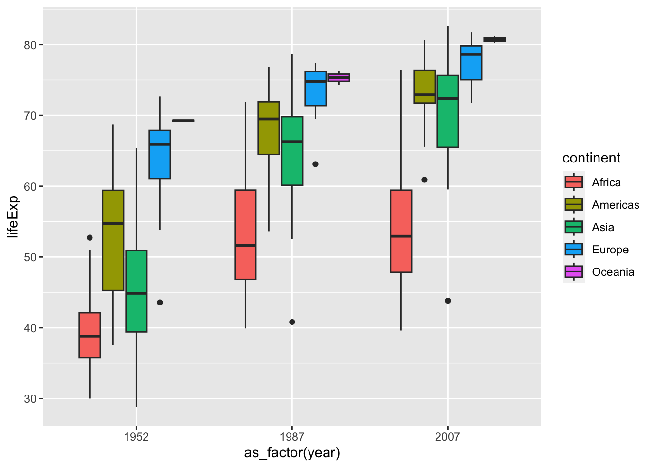
The following are examples of line graphs. Please see the differences.
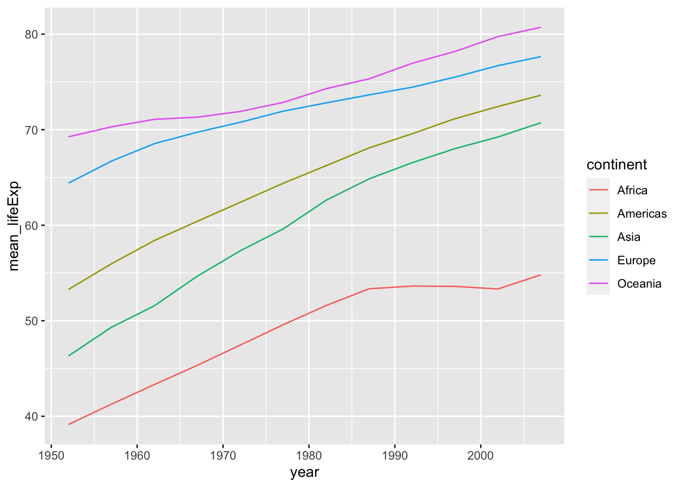
df_lifeExp %>% ggplot(aes(x = year, y = mean_lifeExp, color = continent, linetype = continent)) +
  geom_line()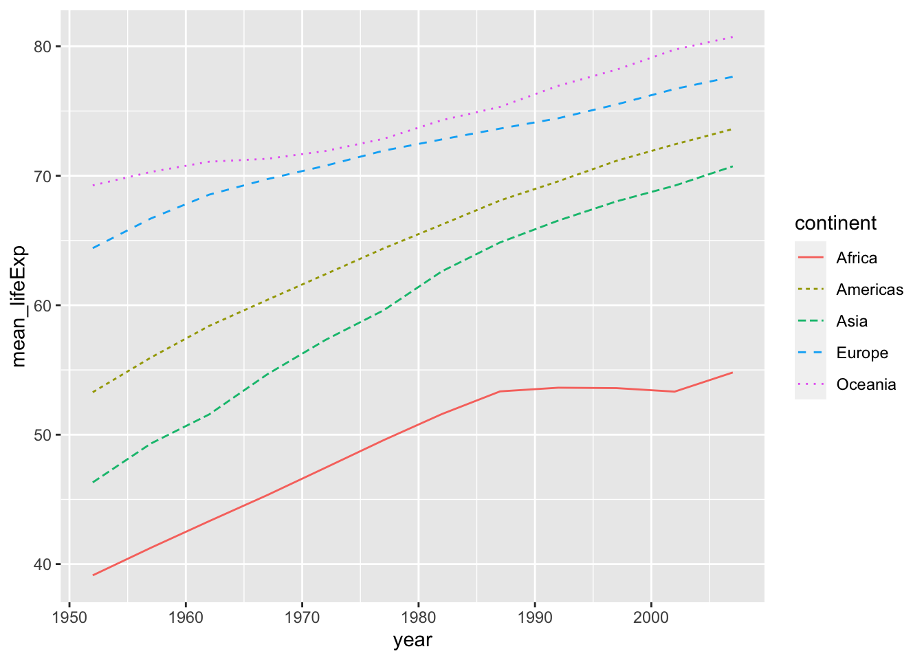
df_lifeExp %>% ggplot() +
  geom_line(aes(x = year, y = mean_lifeExp, color = continent)) +
  geom_line(aes(x = year, y = median_lifeExp, linetype = continent))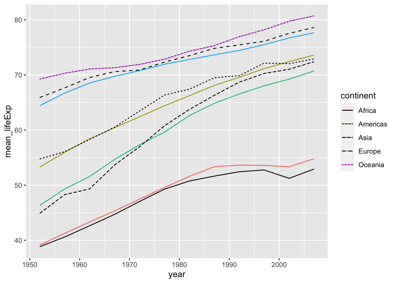
5.11 The Week Two Assignment (in Moodle)
R Markdown and dplyr
- Create an R Notebook of a Data Analysis containing the following and submit the rendered HTML file (eg.
a2_123456.nb.html)- create an R Notebook using the R Notebook Template in Moodle, save as
a2_123456.Rmd, - write your name and ID and the contents,
- run each code block,
- preview to create
a2_123456.nb.html, - submit
a2_123456.nb.htmlto Moodle.
- create an R Notebook using the R Notebook Template in Moodle, save as
-
Pick data from the built-in datasets besides
cars. (library(help = "datasets")or go to the site The R Datasets Package)- Information of the data: Name, Description, Usage, Format, Source, References (Hint: ?cars)
- Use
head(),str(), …, and create at least one chart usingggplot2- Code Chunk.- Don’t forget to add
library(tidyverse)in the first code chunk.
- Don’t forget to add
- An observation of the chart - in your own words.
-
Load
gapminderbylibrary(gapminder).- Choose
poporgdpPercap, or both, one country in the data, a group of countries in the data. - Create charts using ggplot2 with geom_line and the variables and countries chosen in 1. (See examples of the charts for
lifeExp.) - Study the data as you like.
- Observations and difficulties encountered.
- Choose
Due: 2023-01-09 23:59:00. Submit your R Notebook file in Moodle (The Second Assignment). Due on Monday!
5.11.1 Original Data? WDI?
gapminder %>% slice(1:10)
#> # A tibble: 10 × 6
#>    country     continent  year lifeExp      pop gdpPercap
#>    <fct>       <fct>     <int>   <dbl>    <int>     <dbl>
#>  1 Afghanistan Asia       1952    28.8  8425333      779.
#>  2 Afghanistan Asia       1957    30.3  9240934      821.
#>  3 Afghanistan Asia       1962    32.0 10267083      853.
#>  4 Afghanistan Asia       1967    34.0 11537966      836.
#>  5 Afghanistan Asia       1972    36.1 13079460      740.
#>  6 Afghanistan Asia       1977    38.4 14880372      786.
#>  7 Afghanistan Asia       1982    39.9 12881816      978.
#>  8 Afghanistan Asia       1987    40.8 13867957      852.
#>  9 Afghanistan Asia       1992    41.7 16317921      649.
#> 10 Afghanistan Asia       1997    41.8 22227415      635.
5.11.1.1 WDI
- SP.DYN.LE00.IN: Life expectancy at birth, total (years)
- NY.GDP.PCAP.KD: GDP per capita (constant 2015 US$)
- SP.POP.TOTL: Population, total
df_wdi <- WDI(
  country = "all",
  indicator = c(lifeExp = "SP.DYN.LE00.IN", pop = "SP.POP.TOTL", gdpPercap = "NY.GDP.PCAP.KD")
)
#> Rows: 16492 Columns: 7
#> ── Column specification ────────────────────────────────────
#> Delimiter: ","
#> chr (3): country, iso2c, iso3c
#> dbl (4): year, lifeExp, pop, gdpPercap
#>
#> ℹ Use `spec()` to retrieve the full column specification for this data.
#> ℹ Specify the column types or set `show_col_types = FALSE` to quiet this message.
df_wdi %>% slice(1:10)
#> # A tibble: 10 × 7
#>    country     iso2c iso3c  year lifeExp      pop gdpPercap
#>    <chr>       <chr> <chr> <dbl>   <dbl>    <dbl>     <dbl>
#>  1 Afghanistan AF    AFG    1960    32.5  8622466        NA
#>  2 Afghanistan AF    AFG    1961    33.1  8790140        NA
#>  3 Afghanistan AF    AFG    1962    33.5  8969047        NA
#>  4 Afghanistan AF    AFG    1963    34.0  9157465        NA
#>  5 Afghanistan AF    AFG    1964    34.5  9355514        NA
#>  6 Afghanistan AF    AFG    1965    35.0  9565147        NA
#>  7 Afghanistan AF    AFG    1966    35.5  9783147        NA
#>  8 Afghanistan AF    AFG    1967    35.9 10010030        NA
#>  9 Afghanistan AF    AFG    1968    36.4 10247780        NA
#> 10 Afghanistan AF    AFG    1969    36.9 10494489        NA
df_wdi_extra <- WDI(
  country = "all",
  indicator = c(lifeExp = "SP.DYN.LE00.IN", pop = "SP.POP.TOTL", gdpPercap = "NY.GDP.PCAP.KD"),
  extra = TRUE
)
#> Rows: 16492 Columns: 15
#> ── Column specification ────────────────────────────────────
#> Delimiter: ","
#> chr (7): country, iso2c, iso3c, region, capital, income...
#> dbl (6): year, lifeExp, pop, gdpPercap, longitude, lati...
#> lgl (1): status
#> date (1): lastupdated
#>
#> ℹ Use `spec()` to retrieve the full column specification for this data.
#> ℹ Specify the column types or set `show_col_types = FALSE` to quiet this message.
df_wdi_extra
#> # A tibble: 16,492 × 15
#>    country     iso2c iso3c  year status lastupdated lifeExp
#>    <chr>       <chr> <chr> <dbl> <lgl>  <date>        <dbl>
#>  1 Afghanistan AF    AFG    1993 NA     2022-12-22     51.5
#>  2 Afghanistan AF    AFG    1997 NA     2022-12-22     53.6
#>  3 Afghanistan AF    AFG    1994 NA     2022-12-22     51.5
#>  4 Afghanistan AF    AFG    1995 NA     2022-12-22     52.5
#>  5 Afghanistan AF    AFG    2001 NA     2022-12-22     55.8
#>  6 Afghanistan AF    AFG    1998 NA     2022-12-22     52.9
#>  7 Afghanistan AF    AFG    1999 NA     2022-12-22     54.8
#>  8 Afghanistan AF    AFG    2007 NA     2022-12-22     59.1
#>  9 Afghanistan AF    AFG    2008 NA     2022-12-22     59.9
#> 10 Afghanistan AF    AFG    1980 NA     2022-12-22     39.6
#> # ℹ 16,482 more rows
#> # ℹ 8 more variables: pop <dbl>, gdpPercap <dbl>,
#> #   region <chr>, capital <chr>, longitude <dbl>,
#> #   latitude <dbl>, income <chr>, lending <chr>
Can you see the differences? List them out. We will study the World Development Indicators in Chapter 5.11.1.1.