8 `ggplot2`

library(tidyverse)
#> ── Attaching core tidyverse packages ──── tidyverse 2.0.0 ──
#> ✔ dplyr     1.1.3     ✔ readr     2.1.4
#> ✔ forcats   1.0.0     ✔ stringr   1.5.0
#> ✔ ggplot2   3.4.4     ✔ tibble    3.2.1
#> ✔ lubridate 1.9.3     ✔ tidyr     1.3.0
#> ✔ purrr     1.0.2     
#> ── Conflicts ────────────────────── tidyverse_conflicts() ──
#> ✖ dplyr::filter() masks stats::filter()
#> ✖ dplyr::lag()    masks stats::lag()
#> ℹ Use the conflicted package (<http://conflicted.r-lib.org/>) to force all conflicts to become errors

8.1 Learning Resouces

Posit Primers:
- Visualize Data: Learn how to use ggplot2 to make any type of plot with your data. Then learn the best ways to visualize patterns within values and relationships between variables.
r4ds: Data Visualization

8.2 Exploratory Data Analysis

8.2.1 What is EDA?

EDA is an iterative cycle that helps you understand what your data says. When you do EDA, you:

Generate questions about your data
Search for answers by visualising, transforming, and/or modeling your data
Use what you learn to refine your questions and/or generate new questions

EDA is an important part of any data analysis. You can use EDA to make discoveries about the world; or you can use EDA to ensure the quality of your data, asking questions about whether the data meets your standards or not.

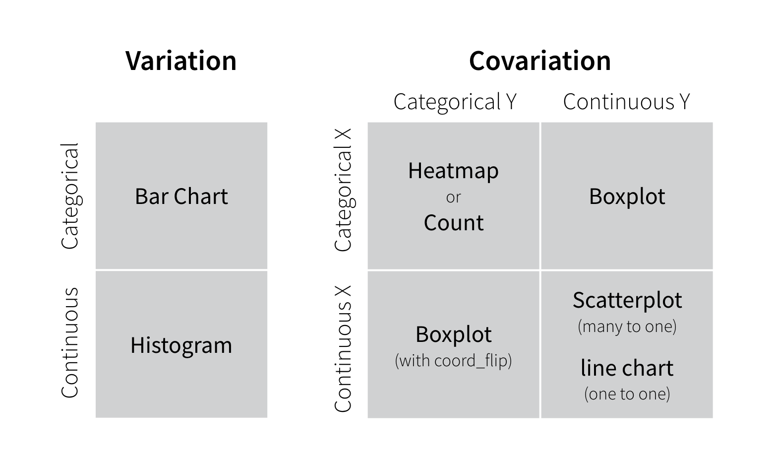
8.2.2 Two useful questions

There is no rule about which questions you should ask to guide your research. However, two types of questions will always be useful for making discoveries within your data. You can loosely word these questions as:

What type of variation occurs within my variables?
What type of covariation occurs between my variables?

The rest of this tutorial will look at these two questions. To make the discussion easier, let’s define some terms…

8.3 Data Visualization

8.4 `ggplot2` Basics

visualization

8.5 Example: World Inequility Report - WIR2022

World Inequality Report: https://wir2022.wid.world/
Executive Summary: https://wir2022.wid.world/executive-summary/
Methodology: https://wir2022.wid.world/methodology/
Data URL: https://wir2022.wid.world/www-site/uploads/2022/03/WIR2022TablesFigures-Summary.xlsx

library(readxl)

url_summary <- "https://wir2022.wid.world/www-site/uploads/2022/03/WIR2022TablesFigures-Summary.xlsx"
download.file(url = url_summary, destfile = "./data/WIR2022s.xlsx", mode = "wb")

excel_sheets("data/WIR2022s.xlsx")
#>  [1] "Index"     "F1"        "F2"        "F3"       
#>  [5] "F4"        "F5."       "F6"        "F7"       
#>  [9] "F8"        "F9"        "F10"       "F11"      
#> [13] "F12"       "F13"       "F14"       "F15"      
#> [17] "T1"        "data-F1"   "data-F2"   "data-F3"  
#> [21] "data-F4"   "data-F5"   "data-F6"   "data-F7"  
#> [25] "data-F8"   "data-F9"   "data-F10"  "data-F11" 
#> [29] "data-F12"  "data-F13." "data-F14." "data-F15"

8.6 F14: Global carbon inequality, 2019. Group contribution to world emissions (%)

Note that the sheet name of F14 has period at the end.

df_f14 <- read_excel("data/WIR2022s.xlsx", sheet = "data-F14.")
df_f14
#> # A tibble: 4 × 2
#>   Group      Share
#>   <chr>      <dbl>
#> 1 Bottom 50% 0.12 
#> 2 Middle 40% 0.404
#> 3 Top 10%    0.476
#> 4 Top 1%     0.168

\n for line break in the title.

8.6.1 Categorical vs Continuous Value

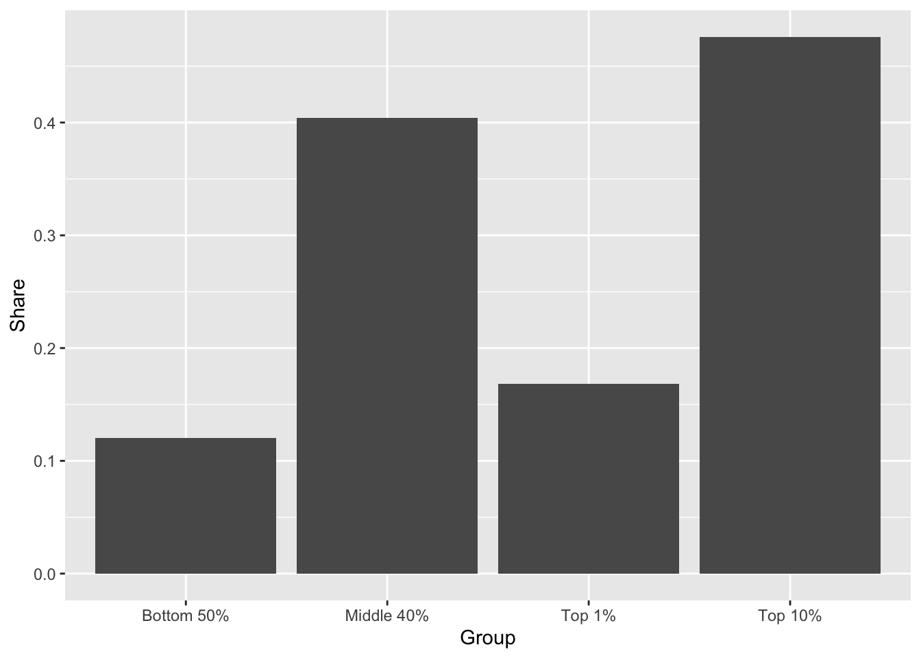
df_f14 %>% 
  ggplot(aes(x = Group, y = Share)) +
  geom_col()

df_f14 %>% 
  ggplot(aes(x = Group, y = Share)) +
  geom_col(width = 0.5, fill = scales::hue_pal()(1)[1]) + 
  scale_y_continuous(labels = scales::percent_format(accuracy = 1)) +
  labs(title = "Figure 14. Global carbon inequality, \n2019 Group contribution to world emissions (%)", 
       x = "", y = "Share of world emissions (%)")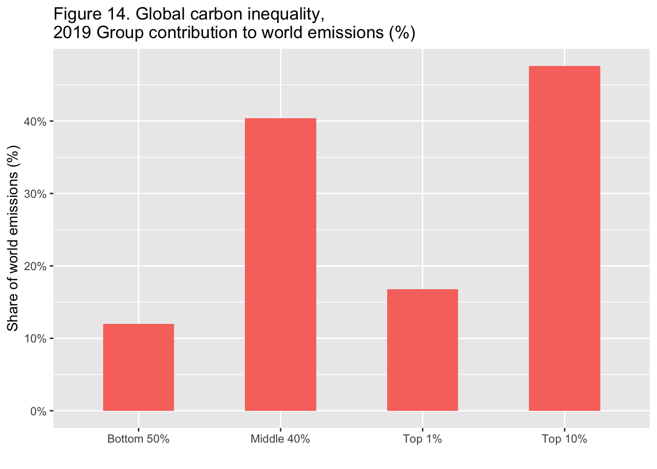

8.6.2 Memo

width = 0.5: width of bars
fill = scales::hue_pal()(1)[1]): hue scale
- https://ggplot2.tidyverse.org/reference/scale_hue.html.
scale_y_continuous(labels = scales::percent_format(accuracy = 1)): percent format
- if accuracy = 0.1, we have 10.0% etc.
labs(title = "Figure 14. Global carbon inequality, \n2019 Group contribution to world emissions (%)", x = "", y = "Share of world emissions (%)")
- title = ““: \n is for line feed
- x, y: labels of x-axis and y-axis

8.7 F12: Female share in global labor incomes, 1990-2020

df_f12 <- read_excel("data/WIR2022s.xlsx", sheet = "data-F12")
#> New names:
#> • `` -> `...2`
df_f12
#> # A tibble: 9 × 2
#>   `Data needs to be updated`   ...2
#>   <chr>                       <dbl>
#> 1 <NA>                       NA    
#> 2 <NA>                       NA    
#> 3 <NA>                       NA    
#> 4 1990                        0.306
#> 5 1995                        0.313
#> 6 2000                        0.325
#> 7 2005                        0.335
#> 8 2010                        0.342
#> 9 2015-2020                   0.347

df_f12 %>% 
  select(year = "Data needs to be updated", value = ...2) %>%
  filter(!is.na(year)) %>%
  ggplot(aes(x = year, y = value)) +
  geom_col(width = 0.5, fill = scales::hue_pal()(2)[2])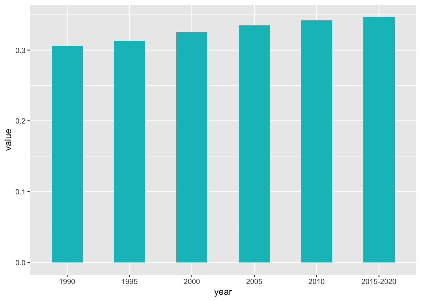

df_f12 %>% 
  select(year = "Data needs to be updated", value = ...2) %>%
  filter(!is.na(year)) %>%
  ggplot(aes(x = year, y = value)) +
  geom_col(width = 0.5, fill = scales::hue_pal()(2)[2]) +
  geom_hline(yintercept = 0.5, linetype = 2, colour = scales::hue_pal()(2)[1]) +
  scale_y_continuous(labels = scales::percent_format(accuracy = 1)) +
  labs(title = "Figure 12. Female share in global labor incomes, 1990-2020", 
        x = "", y = "") +
  annotate("text", x = 1, y = 0.48, label = "Gender parity", size = 3) +
  annotate("text", x = 5.2, y = 0.47, label = stringr::str_wrap("Women make only 35% of global labor incomes, men make the remaining  65%.", width = 40), size = 3)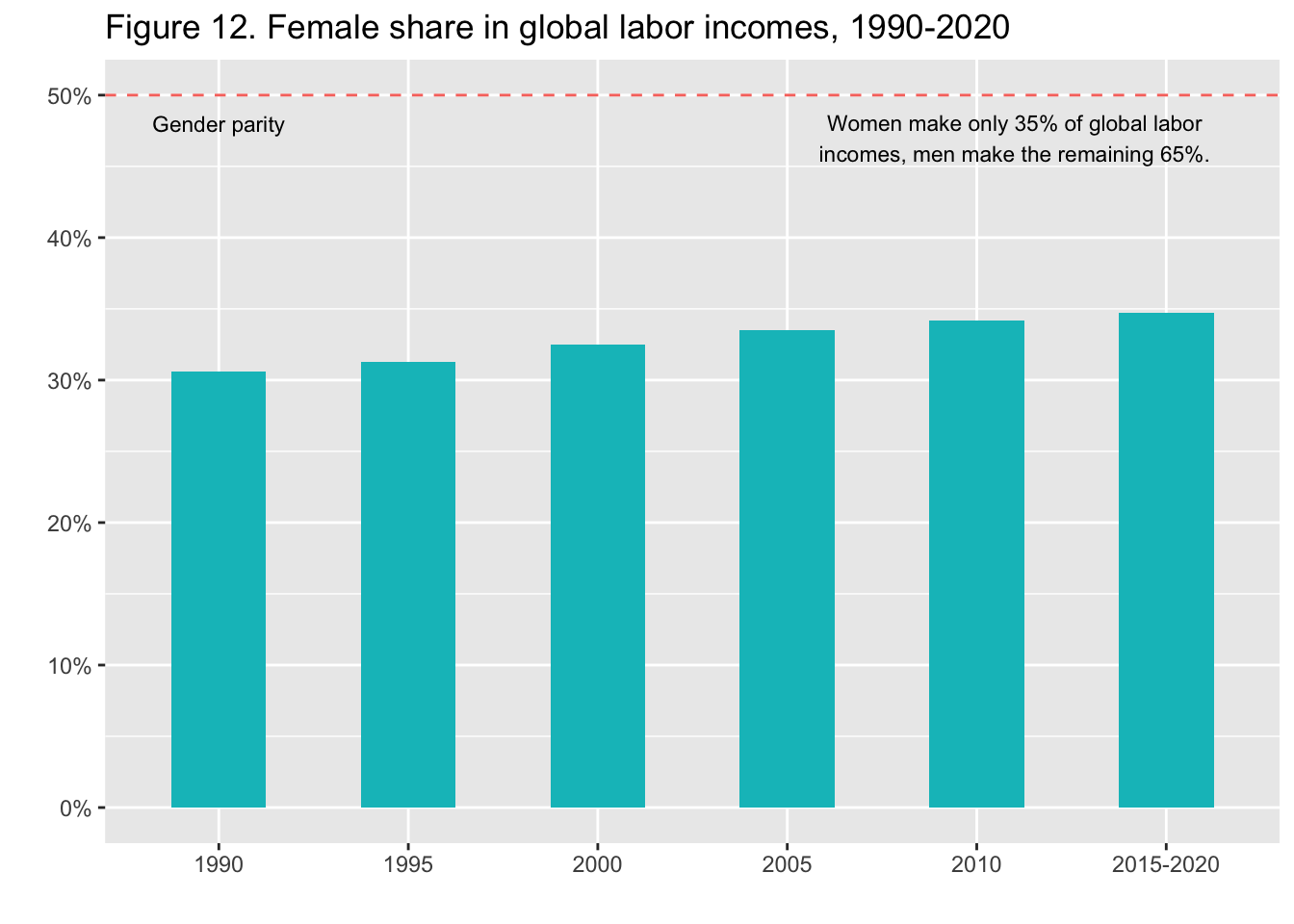

8.8 F1: Global income and wealth inequality, 2021

df_f1 <- read_excel("data/WIR2022s.xlsx", sheet = "data-F1")
#> New names:
#> • `` -> `...1`
df_f1
#> # A tibble: 2 × 5
#>   ...1   `Bottom 50%` `Middle 40%` `Top 10%` `Top 1%`
#>   <chr>         <dbl>        <dbl>     <dbl>    <dbl>
#> 1 Income       0.084         0.394     0.522    0.192
#> 2 Wealth       0.0199        0.224     0.756    0.378

#> # A tibble: 6 × 3
#>   cat    group       value
#>   <chr>  <chr>       <dbl>
#> 1 Income Bottom 50% 0.084 
#> 2 Income Middle 40% 0.394 
#> 3 Income Top 10%    0.522 
#> 4 Wealth Bottom 50% 0.0199
#> 5 Wealth Middle 40% 0.224 
#> 6 Wealth Top 10%    0.756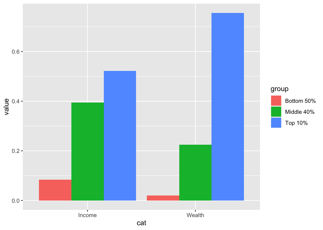

df_f1_rev %>%
  ggplot(aes(x = cat, y = value, fill = group)) +
  geom_col(position = "dodge")

8.9 References of `ggplot2`

Textbook: R for Data Science, Data Visualization

8.9.1 RStudio Primers: See References in Moodle at the bottom

Visualize Data – r4ds: Explore, II

8.10 The Week Three Assignment (in Moodle)

WDI and ggplot2

Create an R Notebook of a Data Analysis containing the following and submit the rendered HTML file (eg. a3_123456.nb.html by replacing 123456 with your ID)
1. create an R Notebook using the R Notebook Template in Moodle, save as a3_123456.Rmd,
2. write your name and ID and the contents,
3. run each code block,
4. preview to create a3_123456.nb.html,
5. submit a3_123456.nb.html to Moodle.

Choose at least one indicator of WDI
- Information of the data: Name, Indicator, Description, Source, etc.
- Download the data with WDI
- Explain why you chose the indicator
- List questions you want to study
Explore the data using visualization using ggplot2
- Use a histogram (geom_histogram), boxplot (geom_boxplot), a scatter plot (geom_point), a line plot (geom_line)
- For at least one chart, add title, and labels of axis, and add an explanation of it
Observations and difficulties encountered.

Due: 2023-01-16 23:59:00. Submit your R Notebook file in Moodle (The Third Assignment). Due on Monday!

7 WDI

9 Assignment Three

8 ggplot2