14 Roudups
library(tidyverse)
#> ── Attaching core tidyverse packages ──── tidyverse 2.0.0 ──
#> ✔ dplyr     1.1.3     ✔ readr     2.1.4
#> ✔ forcats   1.0.0     ✔ stringr   1.5.0
#> ✔ ggplot2   3.4.4     ✔ tibble    3.2.1
#> ✔ lubridate 1.9.3     ✔ tidyr     1.3.0
#> ✔ purrr     1.0.2
#> ── Conflicts ────────────────────── tidyverse_conflicts() ──
#> ✖ dplyr::filter() masks stats::filter()
#> ✖ dplyr::lag()    masks stats::lag()
#> ℹ Use the conflicted package (<http://conflicted.r-lib.org/>) to force all conflicts to become errors
14.1 R Markdown Revisited
Presentation: Submit an R Notebook (with codes used in the presentation), and PowerPoint file or other files used for your presentation, if any. If you use R Notebook for your presentation, you do not need to submit extra files.
Final Paper: Submit an R Notebook (with codes as a work file), and a PDF (rendered directly from an R Notebook, or created from Word) - Maximum pages of PDF is eight.
Format of Presentation - R Notebook is fine and slide presentation in various format is also fine
14.1.1 Literate Programming and Reproducible Research
Importing Data:
- Read a csv file:
read_csv("./data/file_name.csv") - Download and import using a url of a csv file:
read_csv(url) - Read an Excel file:
readxl::read_excel("./data/excel_file_name.xlsx") - Read from the clipboard:
read_delim(clipboard())
- zip file:
copy the url
wir1to10 <- “https://wir2022.wid.world/www-site/uploads/2022/03/WIR2022TablesFigures-Chapter.zip”
download.file(wir1to10, destfile = “./data/wir1to10.zip”)
unzip(“./data/wir1to10.zip”, exdir = “./data”)
list.files(“./data/WIR2022TablesFigures-Chapter”)
excel_sheets(“./data/WIR2022TablesFigures-Chapter/WIR2022TablesFigures-Chapter1.xlsx”)
df <- read_delim(clipboard()); df
Not reproducible unless clearly explained.
14.1.2 Code Chunk Options
https://yihui.org/knitr/options/
Chunk Name
-
Output: use document default
- Show code and output: echo=TRUE, eval=TRUE - Default
- Show output only: echo=FALSE
- Show nothing (run code): include=FALSE
- Show nothing (don’t run code): include=FALSE, eval=FALSE
Show message: message=TRUE, FALSE
Show warning: warning=TRUE, FALSE
Use Paged Tables: paged.print=TRUE, FALSE
Use custom figure size: width and height in inch.
You can use Hide Code and Show Code option on the rendered Notebook file.
14.1.3 Presentation and Paper
Data Source
Variables
Problems
Visualization
Model
-
Conclusions and Further Research
WDI, WIR, etc
14.1.4 Word
Custom Word templates: https://bookdown.org/yihui/rmarkdown-cookbook/word-template.html
You can apply the styles defined in a Word template document to new Word documents generated from R Markdown. Such a template document is also called a “style reference document.” The key is that you have to create this template document from Pandoc first, and change the style definitions in it later. Then pass the path of this template to the reference_docx option of word_document
---
 word_document:
    reference_docx: "template.docx"
---
14.1.5 PowerPoint
PowerPoint presentation: https://bookdown.org/yihui/rmarkdown/powerpoint-presentation.html
Custom templates: https://bookdown.org/yihui/rmarkdown/powerpoint-presentation.html#ppt-templates
---
  powerpoint_presentation:
    reference_doc: my-styles.pptx
---YouTube: How To Create A PowerPoint Template
14.2 The Week Six Assignment - Assignment Five (in Moodle)
- Choose a public data. Clearly state how you obtained the data. Even if you are able to give the URL to download the data, explain the steps you reached and obtained the data.
- Create an R Notebook of a Data Analysis containing the following and submit the rendered HTML file (eg.
a5_123456.nb.htmlby replacing 123456 with your ID), and a PDF (or MS Word File).- create an R Notebook using the R Notebook Template in Moodle, save as
a3_123456.Rmd, - write your name and ID and the contents,
- run each code block,
- preview to create
a5_123456.nb.html, - render (or knit) PDF, or Word (and then PDF)
- submit
a5_123456.nb.htmland PDF (or Word) to Moodle.
- create an R Notebook using the R Notebook Template in Moodle, save as
-
Choose a data with at least two numerical variables. One of them can be the year.
- Information of the data
- Explain why you chose the data
- List questions you want to study
-
Explore the data using visualization using
ggplot2- Create various charts, and write observed comments
- Apply a (linear regression) model, and draw a regression line to at least one chart, and write your conclusion based on the model using the slope value and R squared (and/or adjusted R squared).
Observations based on your data visualization, and difficulties and questions encountered if any.
Due: 2023-01-30 23:59:00. Submit your R Notebook file, and a PDF file (or a MS Word file) in Moodle (The Fifth Assignment). Due on Monday!
14.3 Roundup
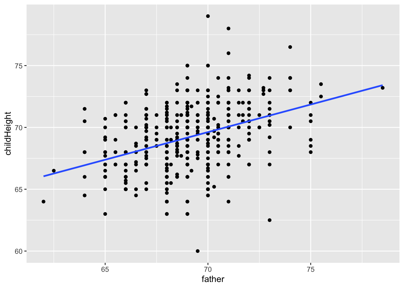
14.3.1 History of Regression Analysis: slope = 0.4465
The heights of descendants of tall ancestors tend to regress down towards a normal average

14.3.2 Anna Karenina Principle
“Tidy data sets are all alike; but every messy data set is messy in its own way.” — Hadley Wickham
“all happy families are all alike; each unhappy family is unhappy in its own way” - Tolstoy’s Anna Karenina
The Anna Karenina principle states that a deficiency in any one of a number of factors dooms an endeavor to failure. Consequently, a successful endeavor (subject to this principle) is one for which every possible deficiency has been avoided. (Wikipedia)
Please look at the outliers carefully.