9 Assignment Three
Assignment Three: The Week Four Assignment
WDI and ggplot2
- Create an R Notebook of a Data Analysis containing the following and submit the rendered HTML file (eg.
a3_123456.nb.htmlby replacing 123456 with your ID)- create an R Notebook using the R Notebook Template in Moodle, save as
a3_123456.Rmd, - write your name and ID and the contents,
- run each code block,
- preview to create
a3_123456.nb.html, - submit
a3_123456.nb.htmlto Moodle.
- create an R Notebook using the R Notebook Template in Moodle, save as
-
Choose at least one indicator of WDI
- Information of the data: Name, Indicator, Description, Source, etc.
- Download the data with
WDI - Explain why you chose the indicator
- List questions you want to study
-
Explore the data using visualization using
ggplot2- Use a histogram (geom_histogram), boxplot (geom_boxplot), a scatter plot (geom_point), a line plot (geom_line)
- For at least one chart, add title, and labels of axis, and add an explanation of it
Observations and difficulties encountered.
Due: 2023-01-16 23:59:00. Submit your R Notebook file in Moodle (The Third Assignment). Due on Monday!
9.1 Set up
Follow the workflow explained in EDA4 on January 18.
9.1.1 EDA by R Studio: Step 1
In RStudio,
1.1. Project
- Create a new project: File > New Project; or
- Open a project: File > Open Project, Open Project in New Session, Open Recent Project
- It is easier to find an existing project from: File > Recent Project
- Check there is a file
project_name.Rprojin your project folder (directory)
1.2. data folder (directory) data
- Create a data folder: Press New Folder at the right bottom pane; or
- Confirm the data folder previously created: Press Files at the right bottom pane
- If you follow 1, the data folder exists in your project folder
1.3. Move (or copy) data for the project to the data folder
- If you downloaded the data, it is in your Download folder. Move it to
data. - Check in your RStudio that your data is in
data: Press Files at the right bottom pane and clickdata, the data folder.
9.1.2 EDA by R Studio: Step 2
2.1. Project Notebook: Memo
-
Create an R Notebook: File > New File > R Notebook
- You can use R Notebook template in Moodle by moving the template (template.Rmd or template.nb.Rmd) file in your project folder or copy and paste the text file into your new R Notebook.
- If you use template.nb.Rmd (R Notebook File), choose Open in Editor.
Add descriptive title.
2.2. Setup Code Chunk
-
Create a code chunk and add packages to use in the project and RUN the code.
- library(tidyverse)
- library(WDI)
- or any other packages
library(tidyverse)
#> ── Attaching core tidyverse packages ──── tidyverse 2.0.0 ──
#> ✔ dplyr     1.1.3     ✔ readr     2.1.4
#> ✔ forcats   1.0.0     ✔ stringr   1.5.0
#> ✔ ggplot2   3.4.4     ✔ tibble    3.2.1
#> ✔ lubridate 1.9.3     ✔ tidyr     1.3.0
#> ✔ purrr     1.0.2
#> ── Conflicts ────────────────────── tidyverse_conflicts() ──
#> ✖ dplyr::filter() masks stats::filter()
#> ✖ dplyr::lag()    masks stats::lag()
#> ℹ Use the conflicted package (<http://conflicted.r-lib.org/>) to force all conflicts to become errors
library(WDI)
When people read a paper, they want to know the minimal set of packages required to install. So it is better to load the packages by library() you actually need in the paper.
2.3. Choose Source or Visual editor mode, and start editing Project Notebook
- Set up Headings such as: About, Data, Analysis and Visualizations, Conclusions
- Under About or Data, paste url of the sites and/or the data
2.4. Edit a new file by saving as for a report
- File > Save As…
9.2 General Comments
9.3 World Development Indicators (WDI)
9.3.1 Setup
It is not a must, but it is good to run the following code chunk and use wdi_cache for WDIsearch() to update the mata data. See WDIcache help.
wdi_cache <- WDIcache()9.3.2 Indicators Used in Assignment Three
- NY.GDP.PCAP.KD: GDP per capita (constant 2015 US$)
- NY.GDP.MKTP.CD: GDP (current US$)
- NY.GDP.PCAP.KD.ZG: GDP per capita growth (annual%)
- SP.POP.TOTL: Total Population
- IP.JRN.ARTC.SC: Scientific and technical journal articles
- FP.CPI.TOTL.ZG: Inflation, consumer prices (% annual growth)
- DT.ODA.ODAT.PC.ZS: Net ODA received per capita (current US$)
- BX.KLT.DINV.CD.WD: Foreign direct investment, net inflows (BoP, current US$)
- MS.MIL.XPND.GD.ZS: Military expenditure (% of GDP)
- MS.MIL.TOTL.P1: Total Armed Forces Personnel
- SI.POV.MDIM: Multidimensional poverty headcount ratio (% of total population)
- SI.POV.NAHC: Poverty headcount ratio at national poverty lines (% of population)
- SI.POV.GINI: Gini index
- NY.GNS.ICTR.ZS: Gross savings (% of GDP)
- SL.UEM.TOTL.ZS: Unemployment, total (% of total labor force) (modeled ILO estimate)
- SP.URB.TOTL.IN.ZS (Urban population (% of total population))
- AG.LND.AGRI.ZS: Agricultural land (% of land area)
- SE.ADT.LITR.FE.ZS: Literacy rate, adult female (% of females ages 15 and above))
- SE.ADT.LITR.MA.ZS: Literacy rate, adult male (% of males ages 15 and above))
- SE.ADT.LITR.ZS: Literacy rate, adult total
- SE.ADT.1524.LT.FE.ZS: Literacy rate, youth female (% of females ages 15-24)
- SE.XPD.TOTL.GD.ZS: Government expenditure on education, total (% of GDP)
- SG.GEN.PARL.ZS: Proportion of seats held by women in national parliaments (%)
9.3.3 WDIsearch
We obtain the information of the data, i.e., meta data of WDI: Name, Indicator, Description, Source, etc. by WDIsearch.
- Usage
WDIsearch(string = "gdp", field = "name", short = TRUE, cache = NULL)-
Arguments
string: Character string. Search for this string using grep with ignore.case=TRUE.field: Character string. Search this field. Admissible fields: ‘indicator’, ‘name’, ‘description’, ‘sourceDatabase’, ‘sourceOrganization’short: TRUE: Returns only the indicator’s code and name. FALSE: Returns the indicator’s code, name, description, and source.cache: Data list generated by the WDIcache function. If omitted, WDIsearch will search a local list of series.
If you follow the order of the arguments, you can omit argument names: string, field, short, cache.
- The simplest format 1.
WDIsearch("NY.GNS.ICTR.ZS", "indicator")
#>            indicator                     name
#> 11497 NY.GNS.ICTR.ZS Gross savings (% of GDP)- The simplest format 2.
WDIsearch("Literacy rate", "name")
#>                             indicator
#> 27            1.1_YOUTH.LITERACY.RATE
#> 8841            IN.POV.LIT.RAT.FEMALE
#> 8842              IN.POV.LIT.RAT.MALE
#> 8843              IN.POV.LIT.RAT.RURL
#> 8844  IN.POV.LIT.RAT.SLUMS.FEMALE.PCT
#> 8845    IN.POV.LIT.RAT.SLUMS.MALE.PCT
#> 8846    IN.POV.LIT.RAT.SLUMS.TOTL.PCT
#> 8847              IN.POV.LIT.RAT.TOTL
#> 8848              IN.POV.LIT.RAT.URBN
#> 15160            SE.ADT.1524.IL.FE.ZS
#> 15161            SE.ADT.1524.IL.MA.ZS
#> 15162               SE.ADT.1524.IL.ZS
#> 15163            SE.ADT.1524.LT.FE.ZS
#> 15164            SE.ADT.1524.LT.FM.ZS
#> 15165            SE.ADT.1524.LT.MA.ZS
#> 15166               SE.ADT.1524.LT.ZS
#> 15167               SE.ADT.ILIT.FE.ZS
#> 15168               SE.ADT.ILIT.MA.ZS
#> 15169                  SE.ADT.ILIT.ZS
#> 15170               SE.ADT.LITR.FE.ZS
#> 15171               SE.ADT.LITR.MA.ZS
#> 15172                  SE.ADT.LITR.ZS
#> 15186                 SE.LITR.15UP.ZS
#> 18792           UIS.LR.AG15T24.F.LPIA
#> 18793             UIS.LR.AG15T24.GPIA
#> 18794             UIS.LR.AG15T24.LPIA
#> 18795           UIS.LR.AG15T24.M.LPIA
#> 18796              UIS.LR.AG15T24.RUR
#> 18797            UIS.LR.AG15T24.RUR.F
#> 18798         UIS.LR.AG15T24.RUR.GPIA
#> 18799            UIS.LR.AG15T24.RUR.M
#> 18800              UIS.LR.AG15T24.URB
#> 18801            UIS.LR.AG15T24.URB.F
#> 18802         UIS.LR.AG15T24.URB.GPIA
#> 18803            UIS.LR.AG15T24.URB.M
#> 18804           UIS.LR.AG15T99.F.LPIA
#> 18805             UIS.LR.AG15T99.GPIA
#> 18806             UIS.LR.AG15T99.LPIA
#> 18807           UIS.LR.AG15T99.M.LPIA
#> 18808              UIS.LR.AG15T99.RUR
#> 18809            UIS.LR.AG15T99.RUR.F
#> 18810         UIS.LR.AG15T99.RUR.GPIA
#> 18811            UIS.LR.AG15T99.RUR.M
#> 18812              UIS.LR.AG15T99.URB
#> 18813            UIS.LR.AG15T99.URB.F
#> 18814         UIS.LR.AG15T99.URB.GPIA
#> 18815            UIS.LR.AG15T99.URB.M
#> 18816                  UIS.LR.AG25T64
#> 18817                UIS.LR.AG25T64.F
#> 18818           UIS.LR.AG25T64.F.LPIA
#> 18819             UIS.LR.AG25T64.GPIA
#> 18820             UIS.LR.AG25T64.LPIA
#> 18821                UIS.LR.AG25T64.M
#> 18822           UIS.LR.AG25T64.M.LPIA
#> 18823              UIS.LR.AG25T64.RUR
#> 18824            UIS.LR.AG25T64.RUR.F
#> 18825         UIS.LR.AG25T64.RUR.GPIA
#> 18826            UIS.LR.AG25T64.RUR.M
#> 18827              UIS.LR.AG25T64.URB
#> 18828            UIS.LR.AG25T64.URB.F
#> 18829         UIS.LR.AG25T64.URB.GPIA
#> 18830            UIS.LR.AG25T64.URB.M
#> 18831                     UIS.LR.AG65
#> 18832                   UIS.LR.AG65.F
#> 18833                   UIS.LR.AG65.M
#> 18834           UIS.LR.AG65T99.F.LPIA
#> 18835             UIS.LR.AG65T99.GPIA
#> 18836             UIS.LR.AG65T99.LPIA
#> 18837           UIS.LR.AG65T99.M.LPIA
#> 18838              UIS.LR.AG65T99.RUR
#> 18839            UIS.LR.AG65T99.RUR.F
#> 18840         UIS.LR.AG65T99.RUR.GPIA
#> 18841            UIS.LR.AG65T99.RUR.M
#> 18842              UIS.LR.AG65T99.URB
#> 18843            UIS.LR.AG65T99.URB.F
#> 18844         UIS.LR.AG65T99.URB.GPIA
#> 18845            UIS.LR.AG65T99.URB.M
#>                                                                                             name
#> 27                                          Literacy rate, youth total (% of people ages 15-24)
#> 8841                                                                    Literacy Rate Female (%)
#> 8842                                                                      Literacy Rate Male (%)
#> 8843                                                                    Literacy rate, Rural (%)
#> 8844                                                           Literacy Rate in Slums-Female (%)
#> 8845                                                           Literacy Rate in Slums - Male (%)
#> 8846                                                         Literacy Rate in Slums  - Total (%)
#> 8847                                                                           Literacy Rate (%)
#> 8848                                                                    Literacy rate, Urban (%)
#> 15160                                    Illiteracy rate, youth female (% of females ages 15-24)
#> 15161                                        Illiteracy rate, youth male (% of males ages 15-24)
#> 15162                                      Illiteracy rate, youth total (% of people ages 15-24)
#> 15163                                      Literacy rate, youth female (% of females ages 15-24)
#> 15164                               Literacy rate, youth (ages 15-24), gender parity index (GPI)
#> 15165                                          Literacy rate, youth male (% of males ages 15-24)
#> 15166                                        Literacy rate, youth total (% of people ages 15-24)
#> 15167                             Illiteracy rate, adult female (% of females ages 15 and above)
#> 15168                                 Illiteracy rate, adult male (% of males ages 15 and above)
#> 15169                               Illiteracy rate, adult total (% of people ages 15 and above)
#> 15170                               Literacy rate, adult female (% of females ages 15 and above)
#> 15171                                   Literacy rate, adult male (% of males ages 15 and above)
#> 15172                                 Literacy rate, adult total (% of people ages 15 and above)
#> 15186                    Literacy Rate for Population age 15 and over (in % of total population)
#> 18792 Youth literacy rate, population 15-24 years, female, adjusted location parity index (LPIA)
#> 18793           Youth literacy rate, population 15-24 years, adjusted gender parity index (GPIA)
#> 18794         Youth literacy rate, population 15-24 years, adjusted location parity index (LPIA)
#> 18795   Youth literacy rate, population 15-24 years, male, adjusted location parity index (LPIA)
#> 18796                         Youth literacy rate, population 15-24 years, rural, both sexes (%)
#> 18797                             Youth literacy rate, population 15-24 years, rural, female (%)
#> 18798    Youth literacy rate, population 15-24 years, rural, adjusted gender parity index (GPIA)
#> 18799                               Youth literacy rate, population 15-24 years, rural, male (%)
#> 18800                         Youth literacy rate, population 15-24 years, urban, both sexes (%)
#> 18801                             Youth literacy rate, population 15-24 years, urban, female (%)
#> 18802    Youth literacy rate, population 15-24 years, urban, adjusted gender parity index (GPIA)
#> 18803                               Youth literacy rate, population 15-24 years, urban, male (%)
#> 18804   Adult literacy rate, population 15+ years, female, adjusted location parity index (LPIA)
#> 18805             Adult literacy rate, population 15+ years, adjusted gender parity index (GPIA)
#> 18806           Adult literacy rate, population 15+ years, adjusted location parity index (LPIA)
#> 18807     Adult literacy rate, population 15+ years, male, adjusted location parity index (LPIA)
#> 18808                           Adult literacy rate, population 15+ years, rural, both sexes (%)
#> 18809                               Adult literacy rate, population 15+ years, rural, female (%)
#> 18810      Adult literacy rate, population 15+ years, rural, adjusted gender parity index (GPIA)
#> 18811                                 Adult literacy rate, population 15+ years, rural, male (%)
#> 18812                           Adult literacy rate, population 15+ years, urban, both sexes (%)
#> 18813                               Adult literacy rate, population 15+ years, urban, female (%)
#> 18814      Adult literacy rate, population 15+ years, urban, adjusted gender parity index (GPIA)
#> 18815                                 Adult literacy rate, population 15+ years, urban, male (%)
#> 18816                                      Literacy rate, population 25-64 years, both sexes (%)
#> 18817                                          Literacy rate, population 25-64 years, female (%)
#> 18818       Literacy rate, population 25-64 years, female, adjusted location parity index (LPIA)
#> 18819                 Literacy rate, population 25-64 years, adjusted gender parity index (GPIA)
#> 18820               Literacy rate, population 25-64 years, adjusted location parity index (LPIA)
#> 18821                                            Literacy rate, population 25-64 years, male (%)
#> 18822         Literacy rate, population 25-64 years, male, adjusted location parity index (LPIA)
#> 18823                               Literacy rate, population 25-64 years, rural, both sexes (%)
#> 18824                                   Literacy rate, population 25-64 years, rural, female (%)
#> 18825          Literacy rate, population 25-64 years, rural, adjusted gender parity index (GPIA)
#> 18826                                     Literacy rate, population 25-64 years, rural, male (%)
#> 18827                               Literacy rate, population 25-64 years, urban, both sexes (%)
#> 18828                                   Literacy rate, population 25-64 years, urban, female (%)
#> 18829          Literacy rate, population 25-64 years, urban, adjusted gender parity index (GPIA)
#> 18830                                     Literacy rate, population 25-64 years, urban, male (%)
#> 18831                                Elderly literacy rate, population 65+ years, both sexes (%)
#> 18832                                    Elderly literacy rate, population 65+ years, female (%)
#> 18833                                      Elderly literacy rate, population 65+ years, male (%)
#> 18834 Elderly literacy rate, population 65+ years, female, adjusted location parity index (LPIA)
#> 18835           Elderly literacy rate, population 65+ years, adjusted gender parity index (GPIA)
#> 18836         Elderly literacy rate, population 65+ years, adjusted location parity index (LPIA)
#> 18837   Elderly literacy rate, population 65+ years, male, adjusted location parity index (LPIA)
#> 18838                         Elderly literacy rate, population 65+ years, rural, both sexes (%)
#> 18839                             Elderly literacy rate, population 65+ years, rural, female (%)
#> 18840    Elderly literacy rate, population 65+ years, rural, adjusted gender parity index (GPIA)
#> 18841                               Elderly literacy rate, population 65+ years, rural, male (%)
#> 18842                         Elderly literacy rate, population 65+ years, urban, both sexes (%)
#> 18843                             Elderly literacy rate, population 65+ years, urban, female (%)
#> 18844    Elderly literacy rate, population 65+ years, urban, adjusted gender parity index (GPIA)
#> 18845 Elderly literacy rate, population 65+ years, urban, male (%)- Detailed with short = FALSE
WDIsearch("IP.JRN.ARTC.SC", "indicator", FALSE)
#>           indicator
#> 8885 IP.JRN.ARTC.SC
#>                                           name
#> 8885 Scientific and technical journal articles
#>                                                                                                                                                                                                                                                                              description
#> 8885 Scientific and technical journal articles refer to the number of scientific and engineering articles published in the following fields: physics, biology, chemistry, mathematics, clinical medicine, biomedical research, engineering and technology, and earth and space sciences.
#>                    sourceDatabase
#> 8885 World Development Indicators
#>                                                    sourceOrganization
#> 8885 National Science Foundation, Science and Engineering Indicators.- You can use
wdi_cachedownloaded above to use the updated meta data.
WDIsearch("Government expenditure on education", "name", FALSE, wdi_cache)
#> indicator
#> 16703 SE.XPD.PRIM.ZS
#> 16707 SE.XPD.SECO.ZS
#> 16712 SE.XPD.TERT.ZS
#> 16713 SE.XPD.TOTL.GB.ZS
#> 16714 SE.XPD.TOTL.GD.ZS
#> 20830 UIS.X.PPP.FSGOV
#> 20831 UIS.X.PPP.UK.FSGOV
#> 20840 UIS.X.PPPCONST.FSGOV
#> 20841 UIS.X.PPPCONST.UK.FSGOV
#> 20850 UIS.X.US.FSGOV
#> 20851 UIS.X.US.UK.FSGOV
#> 20860 UIS.X.USCONST.FSGOV
#> 20861 UIS.X.USCONST.UK.FSGOV
#> name
#> 16703 Expenditure on primary education (% of government expenditure on education)
#> 16707 Expenditure on secondary education (% of government expenditure on education)
#> 16712 Expenditure on tertiary education (% of government expenditure on education)
#> 16713 Government expenditure on education, total (% of government expenditure)
#> 16714 Government expenditure on education, total (% of GDP)
#> 20830 Government expenditure on education, PPP$ (millions)
#> 20831 Government expenditure on education not specified by level, PPP$ (millions)
#> 20840 Government expenditure on education, constant PPP$ (millions)
#> 20841 Government expenditure on education not specified by level, constant PPP$ (millions)
#> 20850 Government expenditure on education, US$ (millions)
#> 20851 Government expenditure on education not specified by level, US$ (millions)
#> 20860 Government expenditure on education, constant US$ (millions)
#> 20861 Government expenditure on education not specified by level, constant US$ (millions)
#> description
#> 16703 Expenditure on primary education is expressed as a percentage of total general government expenditure on education. General government usually refers to local, regional and central governments.
#> 16707 Expenditure on secondary education is expressed as a percentage of total general government expenditure on education. General government usually refers to local, regional and central governments.
#> 16712 Expenditure on tertiary education is expressed as a percentage of total general government expenditure on education. General government usually refers to local, regional and central governments.
#> 16713 General government expenditure on education (current, capital, and transfers) is expressed as a percentage of total general government expenditure on all sectors (including health, education, social services, etc.). It includes expenditure funded by transfers from international sources to government. General government usually refers to local, regional and central governments.
#> 16714 General government expenditure on education (current, capital, and transfers) is expressed as a percentage of GDP. It includes expenditure funded by transfers from international sources to government. General government usually refers to local, regional and central governments.
#> 20830 Total general (local, regional and central) government expenditure on education (current, capital, and transfers), in millions PPP$ (at purchasing power parity), in nominal value. It includes expenditure funded by transfers from international sources to government. Total government expenditure for a given level of education (e.g. primary, secondary, or all levels combined) in national currency is converted to PPP$. Limitations: In some instances data on total government expenditure on education refers only to the Ministry of Education, excluding other ministries which may also spend a part of their budget on educational activities. For more information, consult the UNESCO Institute of Statistics website: http://www.uis.unesco.org/Education/
#> 20831 Total general (local, regional and central) government expenditure on education (current, capital, and transfers) not specified by level, in millions PPP$ (at purchasing power parity), in nominal value. It includes expenditure funded by transfers from international sources to government. Total government expenditure for a given level of education (e.g. primary, secondary, or all levels combined) in national currency is converted to PPP$. Limitations: In some instances data on total government expenditure on education refers only to the Ministry of Education, excluding other ministries which may also spend a part of their budget on educational activities. For more information, consult the UNESCO Institute of Statistics website: http://www.uis.unesco.org/Education/
#> 20840 Total general (local, regional and central) government expenditure on education (current, capital, and transfers), in millions PPP$ (at purchasing power parity) in constant value (taking into account inflation). It includes expenditure funded by transfers from international sources to government. Total government expenditure for a given level of education (e.g. primary, secondary, or all levels combined) in national currency is converted to PPP$, and where it is expressed in constant value, uses a GDP deflator to account for inflation. The constant prices base year is normally three years before the year of the data release. For example, in the July 2017 data release, constant PPP$ values are expressed in 2014 prices. Limitations: In some instances data on total government expenditure on education refers only to the Ministry of Education, excluding other ministries which may also spend a part of their budget on educational activities. For more information, consult the UNESCO Institute of Statistics website: http://www.uis.unesco.org/Education/
#> 20841 Total general (local, regional and central) government expenditure on education (current, capital, and transfers) not specified by level, in millions PPP$ (at purchasing power parity) in constant value (taking into account inflation). It includes expenditure funded by transfers from international sources to government. Total government expenditure for a given level of education (e.g. primary, secondary, or all levels combined) in national currency is converted to PPP$, and where it is expressed in constant value, uses a GDP deflator to account for inflation. The constant prices base year is normally three years before the year of the data release. For example, in the July 2017 data release, constant PPP$ values are expressed in 2014 prices. Limitations: In some instances data on total government expenditure on education refers only to the Ministry of Education, excluding other ministries which may also spend a part of their budget on educational activities. For more information, consult the UNESCO Institute of Statistics website: http://www.uis.unesco.org/Education/
#> 20850 Total general (local, regional and central) government expenditure on education (current, capital, and transfers) in millions US$ (nominal value). It includes expenditure funded by transfers from international sources to government. Total government expenditure for a given level of education (e.g. primary, secondary, or all levels combined) in national currency is converted to US$. Limitations: In some instances data on total government expenditure on education refers only to the Ministry of Education, excluding other ministries which may also spend a part of their budget on educational activities. For more information, consult the UNESCO Institute of Statistics website: http://www.uis.unesco.org/Education/
#> 20851 Total general (local, regional and central) government expenditure on education (current, capital, and transfers) not specified by level in millions US$ (nominal value). It includes expenditure funded by transfers from international sources to government. Total government expenditure for a given level of education (e.g. primary, secondary, or all levels combined) in national currency is converted to US$. Limitations: In some instances data on total government expenditure on education refers only to the Ministry of Education, excluding other ministries which may also spend a part of their budget on educational activities. For more information, consult the UNESCO Institute of Statistics website: http://www.uis.unesco.org/Education/
#> 20860 Total general (local, regional and central) government expenditure on education (current, capital, and transfers) in millions US$ in constant value (taking into account inflation). It includes expenditure funded by transfers from international sources to government. Total government expenditure for a given level of education (e.g. primary, secondary, or all levels combined) in national currency is converted to US$, and where it is expressed in constant value, uses a GDP deflator to account for inflation. The constant prices base year is normally three years before the year of the data release. For example, in the July 2017 data release, constant US$ values are expressed in 2014 prices. Limitations: In some instances data on total government expenditure on education refers only to the Ministry of Education, excluding other ministries which may also spend a part of their budget on educational activities. For more information, consult the UNESCO Institute of Statistics website: http://www.uis.unesco.org/Education/
#> 20861 Total general (local, regional and central) government expenditure on education (current, capital, and transfers) not specified by level in millions US$ in constant value (taking into account inflation). It includes expenditure funded by transfers from international sources to government. Total government expenditure for a given level of education (e.g. primary, secondary, or all levels combined) in national currency is converted to US$, and where it is expressed in constant value, uses a GDP deflator to account for inflation. The constant prices base year is normally three years before the year of the data release. For example, in the July 2017 data release, constant US$ values are expressed in 2014 prices. Limitations: In some instances data on total government expenditure on education refers only to the Ministry of Education, excluding other ministries which may also spend a part of their budget on educational activities. For more information, consult the UNESCO Institute of Statistics website: http://www.uis.unesco.org/Education/
#> sourceDatabase
#> 16703 World Development Indicators
#> 16707 World Development Indicators
#> 16712 World Development Indicators
#> 16713 World Development Indicators
#> 16714 World Development Indicators
#> 20830 Education Statistics
#> 20831 Education Statistics
#> 20840 Education Statistics
#> 20841 Education Statistics
#> 20850 Education Statistics
#> 20851 Education Statistics
#> 20860 Education Statistics
#> 20861 Education Statistics
#> sourceOrganization
#> 16703 UNESCO Institute for Statistics (http://uis.unesco.org/). Data as of February 2020.
#> 16707 UNESCO Institute for Statistics (http://uis.unesco.org/). Data as of February 2020.
#> 16712 UNESCO Institute for Statistics (http://uis.unesco.org/). Data as of February 2020.
#> 16713 UNESCO Institute for Statistics (UIS). UIS.Stat Bulk Data Download Service. Accessed October 24, 2022. https://apiportal.uis.unesco.org/bdds.
#> 16714 UNESCO Institute for Statistics (UIS). UIS.Stat Bulk Data Download Service. Accessed October 24, 2022. https://apiportal.uis.unesco.org/bdds.
#> 20830 UNESCO Institute for Statistics
#> 20831 UNESCO Institute for Statistics
#> 20840 UNESCO Institute for Statistics
#> 20841 UNESCO Institute for Statistics
#> 20850 UNESCO Institute for Statistics
#> 20851 UNESCO Institute for Statistics
#> 20860 UNESCO Institute for Statistics
#> 20861 UNESCO Institute for Statistics9.3.4 Importing Data Using WDI
- The shortest form. The following is same as:
WDI(country = "all", indicator = "NY.GDP.PCAP.KD", start = 1960, end = NULL, extra = FALSE, cache = NULL, latest = NULL, language = "en)
WDI(indicator = "NY.GDP.PCAP.KD")#> Rows: 16492 Columns: 5
#> ── Column specification ────────────────────────────────────
#> Delimiter: ","
#> chr (3): country, iso2c, iso3c
#> dbl (2): year, NY.GDP.PCAP.KD
#>
#> ℹ Use `spec()` to retrieve the full column specification for this data.
#> ℹ Specify the column types or set `show_col_types = FALSE` to quiet this message.
#> # A tibble: 16,492 × 5
#> country iso2c iso3c year NY.GDP.PCAP.KD
#> <chr> <chr> <chr> <dbl> <dbl>
#> 1 Africa Eastern and Sout… ZH AFE 2021 1461.
#> 2 Africa Eastern and Sout… ZH AFE 2020 1437.
#> 3 Africa Eastern and Sout… ZH AFE 2019 1520.
#> 4 Africa Eastern and Sout… ZH AFE 2018 1529.
#> 5 Africa Eastern and Sout… ZH AFE 2017 1532.
#> 6 Africa Eastern and Sout… ZH AFE 2016 1533.
#> 7 Africa Eastern and Sout… ZH AFE 2015 1541.
#> 8 Africa Eastern and Sout… ZH AFE 2014 1538.
#> 9 Africa Eastern and Sout… ZH AFE 2013 1520.
#> 10 Africa Eastern and Sout… ZH AFE 2012 1499.
#> # ℹ 16,482 more rows- In order to use the downloaded data, we need to assign a name to it. It can be
dfif you download and use only one data, but it is better to assign the data to be a more descriptive name.
df_gdppcap <- WDI(indicator = "NY.GDP.PCAP.KD")
df_gdppcap
#> Rows: 16492 Columns: 5
#> ── Column specification ────────────────────────────────────
#> Delimiter: ","
#> chr (3): country, iso2c, iso3c
#> dbl (2): year, NY.GDP.PCAP.KD
#>
#> ℹ Use `spec()` to retrieve the full column specification for this data.
#> ℹ Specify the column types or set `show_col_types = FALSE` to quiet this message.
#> # A tibble: 16,492 × 5
#> country iso2c iso3c year NY.GDP.PCAP.KD
#> <chr> <chr> <chr> <dbl> <dbl>
#> 1 Africa Eastern and Sout… ZH AFE 2021 1461.
#> 2 Africa Eastern and Sout… ZH AFE 2020 1437.
#> 3 Africa Eastern and Sout… ZH AFE 2019 1520.
#> 4 Africa Eastern and Sout… ZH AFE 2018 1529.
#> 5 Africa Eastern and Sout… ZH AFE 2017 1532.
#> 6 Africa Eastern and Sout… ZH AFE 2016 1533.
#> 7 Africa Eastern and Sout… ZH AFE 2015 1541.
#> 8 Africa Eastern and Sout… ZH AFE 2014 1538.
#> 9 Africa Eastern and Sout… ZH AFE 2013 1520.
#> 10 Africa Eastern and Sout… ZH AFE 2012 1499.
#> # ℹ 16,482 more rows- If you want to use extra information such as
region,income,lending, useextra = TRUE.
df_gdppcap_extra <- WDI(indicator = "NY.GDP.PCAP.KD", extra = TRUE)
df_gdppcap_extra
#> Rows: 16492 Columns: 13
#> ── Column specification ────────────────────────────────────
#> Delimiter: ","
#> chr (7): country, iso2c, iso3c, region, capital, income...
#> dbl (4): year, NY.GDP.PCAP.KD, longitude, latitude
#> lgl (1): status
#> date (1): lastupdated
#>
#> ℹ Use `spec()` to retrieve the full column specification for this data.
#> ℹ Specify the column types or set `show_col_types = FALSE` to quiet this message.
#> # A tibble: 16,492 × 13
#> country iso2c iso3c year NY.GDP.PCAP.KD status
#> <chr> <chr> <chr> <dbl> <dbl> <lgl>
#> 1 Afghanistan AF AFG 2015 592. NA
#> 2 Afghanistan AF AFG 2011 551. NA
#> 3 Afghanistan AF AFG 2014 603. NA
#> 4 Afghanistan AF AFG 2013 608. NA
#> 5 Afghanistan AF AFG 2012 596. NA
#> 6 Afghanistan AF AFG 2007 429. NA
#> 7 Afghanistan AF AFG 2010 569. NA
#> 8 Afghanistan AF AFG 2009 512. NA
#> 9 Afghanistan AF AFG 2008 437. NA
#> 10 Afghanistan AF AFG 2003 363. NA
#> # ℹ 16,482 more rows
#> # ℹ 7 more variables: lastupdated <date>, region <chr>,
#> # capital <chr>, longitude <dbl>, latitude <dbl>,
#> # income <chr>, lending <chr>9.3.5 Writing and reading a csv file
Since the data is generally huge, it is better to use a data saved in your computer.
Before saving it check whether you have data folder (or directory) in you project folder. Use the Files tab of the right bottom pane. You should be able to see the project icon with Rproj at the end, your R Notebook file you are editing, and the data folder. Since .csv is automatically added, write_csv(gdppcap_extra, "./data/gdppcap_extra") does the same as below.
write_csv(df_gdppcap_extra, "./data/gdppcap_extra.csv")To read the data, run the next code chunk. You do not have to run the code df_gdppcap_extra <- WDI(indicator = "NY.GDP.PCAP.KD", extra = TRUE) again.
gdppcap <- read_csv("./data/gdppcap_extra.csv")“./data/gdpcap_extra.csv” is the way to express the name of the data gdpcap_extra.csv in csv format in the data folder.
9.3.6 country argument
If you want to import data for several countries, you can use iso2c codes of the countries.
ASEAN <- c("BN", "ID", "KH", "LA", "MM", "MY", "PH", "SG")
df_gdppcap_asean <- WDI(ASEAN, "NY.GDP.PCAP.KD")#> Rows: 496 Columns: 5
#> ── Column specification ────────────────────────────────────
#> Delimiter: ","
#> chr (3): country, iso2c, iso3c
#> dbl (2): year, NY.GDP.PCAP.KD
#>
#> ℹ Use `spec()` to retrieve the full column specification for this data.
#> ℹ Specify the column types or set `show_col_types = FALSE` to quiet this message.
#> # A tibble: 496 × 5
#> country iso2c iso3c year NY.GDP.PCAP.KD
#> <chr> <chr> <chr> <dbl> <dbl>
#> 1 Brunei Darussalam BN BRN 2021 29673.
#> 2 Brunei Darussalam BN BRN 2020 30402.
#> 3 Brunei Darussalam BN BRN 2019 30314.
#> 4 Brunei Darussalam BN BRN 2018 29438.
#> 5 Brunei Darussalam BN BRN 2017 29696.
#> 6 Brunei Darussalam BN BRN 2016 29601.
#> 7 Brunei Darussalam BN BRN 2015 30682.
#> 8 Brunei Darussalam BN BRN 2014 31156.
#> 9 Brunei Darussalam BN BRN 2013 32342.
#> 10 Brunei Darussalam BN BRN 2012 33457.
#> # ℹ 486 more rows
df_gdppcap_asean %>% distinct(country) %>% pull()
#> [1] "Brunei Darussalam" "Indonesia"
#> [3] "Cambodia"          "Lao PDR"
#> [5] "Myanmar"           "Malaysia"
#> [7] "Philippines"       "Singapore"
wdi_cache$country %>% filter(iso2c %in% ASEAN) %>% distinct(country) %>% pull()
#> [1] "Brunei Darussalam" "Indonesia"
#> [3] "Cambodia"          "Lao PDR"
#> [5] "Myanmar"           "Malaysia"
#> [7] "Philippines"       "Singapore"
You can also use wdi_cache$country.
wdi_cache$country %>% slice(1:10)
#>    iso3c iso2c                     country
#> 1    ABW    AW                       Aruba
#> 2    AFE    ZH Africa Eastern and Southern
#> 3    AFG    AF                 Afghanistan
#> 4    AFR    A9                      Africa
#> 5    AFW    ZI  Africa Western and Central
#> 6    AGO    AO                      Angola
#> 7    ALB    AL                     Albania
#> 8    AND    AD                     Andorra
#> 9    ARB    1A                  Arab World
#> 10   ARE    AE        United Arab Emirates
#>                        region          capital longitude
#> 1   Latin America & Caribbean       Oranjestad  -70.0167
#> 2                  Aggregates
#> 3                  South Asia            Kabul   69.1761
#> 4                  Aggregates
#> 5                  Aggregates
#> 6          Sub-Saharan Africa           Luanda    13.242
#> 7       Europe & Central Asia           Tirane   19.8172
#> 8       Europe & Central Asia Andorra la Vella    1.5218
#> 9                  Aggregates
#> 10 Middle East & North Africa        Abu Dhabi   54.3705
#>    latitude              income        lending
#> 1   12.5167         High income Not classified
#> 2                    Aggregates     Aggregates
#> 3   34.5228          Low income            IDA
#> 4                    Aggregates     Aggregates
#> 5                    Aggregates     Aggregates
#> 6  -8.81155 Lower middle income           IBRD
#> 7   41.3317 Upper middle income           IBRD
#> 8   42.5075         High income Not classified
#> 9                    Aggregates     Aggregates
#> 10  24.4764         High income Not classified
wdi_cache$country %>% filter(iso2c %in% ASEAN) %>% pull(country)
#> [1] "Brunei Darussalam" "Indonesia"
#> [3] "Cambodia"          "Lao PDR"
#> [5] "Myanmar"           "Malaysia"
#> [7] "Philippines"       "Singapore"
You can find iso2c codes from the downloaded data, or using wdi_cache$country
wdi_cache$country %>%
  filter(country %in% c("Brunei Darussalam", "Indonesia", "Cambodia", "Lao PDR", "Myanmar", "Malaysia", "Philippines", "Singapore")) %>%
  pull(iso2c)
#> [1] "BN" "ID" "KH" "LA" "MM" "MY" "PH" "SG"
You can also find countries in some category.
wdi_cache$country %>%
  filter(region == "South Asia") %>%
  pull(country)
#> [1] "Afghanistan" "Bangladesh"  "Bhutan"      "India"
#> [5] "Sri Lanka"   "Maldives"    "Nepal"       "Pakistan"
wdi_cache$country %>%
  filter(income == "Lower middle income") %>%
  pull(iso2c)
#>  [1] "AO" "BJ" "BD" "BO" "BT" "CI" "CM" "CG" "KM" "CV" "DJ"
#> [12] "DZ" "EG" "FM" "GH" "HN" "HT" "ID" "IN" "IR" "KE" "KG"
#> [23] "KH" "KI" "LA" "LB" "LK" "LS" "MA" "MM" "MN" "MR" "NG"
#> [34] "NI" "NP" "PK" "PH" "PG" "PS" "SN" "SB" "SV" "ST" "SZ"
#> [45] "TJ" "TL" "TN" "TZ" "UA" "UZ" "VN" "VU" "WS" "ZW"
The following shows a list of indicators
wdi_cache$series %>% slice(1:10)
#>               indicator
#> 1    1.0.HCount.1.90usd
#> 2     1.0.HCount.2.5usd
#> 3  1.0.HCount.Mid10to50
#> 4       1.0.HCount.Ofcl
#> 5   1.0.HCount.Poor4uds
#> 6   1.0.HCount.Vul4to10
#> 7      1.0.PGap.1.90usd
#> 8       1.0.PGap.2.5usd
#> 9     1.0.PGap.Poor4uds
#> 10     1.0.PSev.1.90usd
#>                                       name
#> 1          Poverty Headcount ($1.90 a day)
#> 2          Poverty Headcount ($2.50 a day)
#> 3    Middle Class ($10-50 a day) Headcount
#> 4  Official Moderate Poverty Rate-National
#> 5             Poverty Headcount ($4 a day)
#> 6       Vulnerable ($4-10 a day) Headcount
#> 7                Poverty Gap ($1.90 a day)
#> 8                Poverty Gap ($2.50 a day)
#> 9                   Poverty Gap ($4 a day)
#> 10          Poverty Severity ($1.90 a day)
#>                                                                                                                                                                                                                                                                    description
#> 1                                                                                                                                     The poverty headcount index measures the proportion of the population with daily per capita income (in 2011 PPP) below the poverty line.
#> 2                                                                                                                                     The poverty headcount index measures the proportion of the population with daily per capita income (in 2005 PPP) below the poverty line.
#> 3                                                                                                                                     The poverty headcount index measures the proportion of the population with daily per capita income (in 2005 PPP) below the poverty line.
#> 4                                                                                                                The poverty headcount index measures the proportion of the population with daily per capita income below the official poverty line developed by each country.
#> 5                                                                                                                                     The poverty headcount index measures the proportion of the population with daily per capita income (in 2005 PPP) below the poverty line.
#> 6                                                                                                                                     The poverty headcount index measures the proportion of the population with daily per capita income (in 2005 PPP) below the poverty line.
#> 7  The poverty gap captures the mean aggregate income or consumption shortfall relative to the poverty line across the entire population. It measures the total resources needed to bring all the poor to the level of the poverty line (averaged over the total population).
#> 8  The poverty gap captures the mean aggregate income or consumption shortfall relative to the poverty line across the entire population. It measures the total resources needed to bring all the poor to the level of the poverty line (averaged over the total population).
#> 9  The poverty gap captures the mean aggregate income or consumption shortfall relative to the poverty line across the entire population. It measures the total resources needed to bring all the poor to the level of the poverty line (averaged over the total population).
#> 10                                                                                                        The poverty severity index combines information on both poverty and inequality among the poor by averaging the squares of the poverty gaps relative the poverty line
#>    sourceDatabase
#> 1  LAC Equity Lab
#> 2  LAC Equity Lab
#> 3  LAC Equity Lab
#> 4  LAC Equity Lab
#> 5  LAC Equity Lab
#> 6  LAC Equity Lab
#> 7  LAC Equity Lab
#> 8  LAC Equity Lab
#> 9  LAC Equity Lab
#> 10 LAC Equity Lab
#>                                                       sourceOrganization
#> 1      LAC Equity Lab tabulations of SEDLAC (CEDLAS and the World Bank).
#> 2      LAC Equity Lab tabulations of SEDLAC (CEDLAS and the World Bank).
#> 3      LAC Equity Lab tabulations of SEDLAC (CEDLAS and the World Bank).
#> 4  LAC Equity Lab tabulations of data from National Statistical Offices.
#> 5      LAC Equity Lab tabulations of SEDLAC (CEDLAS and the World Bank).
#> 6      LAC Equity Lab tabulations of SEDLAC (CEDLAS and the World Bank).
#> 7      LAC Equity Lab tabulations of SEDLAC (CEDLAS and the World Bank).
#> 8      LAC Equity Lab tabulations of SEDLAC (CEDLAS and the World Bank).
#> 9      LAC Equity Lab tabulations of SEDLAC (CEDLAS and the World Bank).
#> 10     LAC Equity Lab tabulations of SEDLAC (CEDLAS and the World Bank).
The following is same as WDIsearch("gdp per cap", "name"). See WDIsearch help.
9.4 Responses to Questions
9.4.1 Q1. How do we use histograms.
wdi_cache$series %>% filter(indicator == "SG.GEN.PARL.ZS") %>% pull(name)
#> [1] "Proportion of seats held by women in national parliaments (%)"#> Rows: 5675 Columns: 5
#> ── Column specification ────────────────────────────────────
#> Delimiter: ","
#> chr (3): country, iso2c, iso3c
#> dbl (2): year, women_in_parl
#>
#> ℹ Use `spec()` to retrieve the full column specification for this data.
#> ℹ Specify the column types or set `show_col_types = FALSE` to quiet this message.
df_women_in_parl %>% filter(year == 2020) %>%
  ggplot(aes(women_in_parl)) + geom_histogram()
#> `stat_bin()` using `bins = 30`. Pick better value with
#> `binwidth`.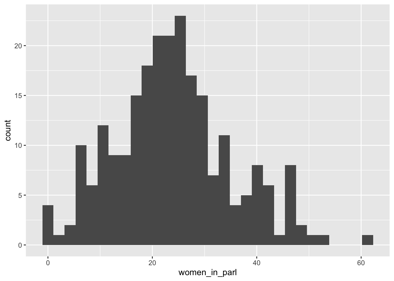
df_women_in_parl %>% filter(year == 2020) %>%
  ggplot(aes(women_in_parl)) + geom_histogram(binwidth = 5)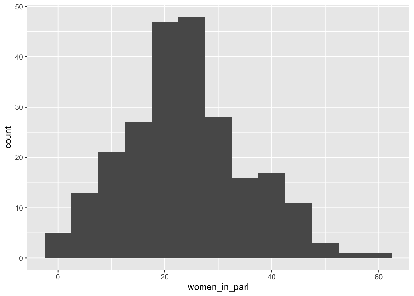
wdi_cache$series %>% filter(indicator == "IP.JRN.ARTC.SC") %>% pull(name)
#> [1] "Scientific and technical journal articles"#> Rows: 4655 Columns: 13
#> ── Column specification ────────────────────────────────────
#> Delimiter: ","
#> chr (7): country, iso2c, iso3c, region, capital, income...
#> dbl (4): year, stja, longitude, latitude
#> lgl (1): status
#> date (1): lastupdated
#>
#> ℹ Use `spec()` to retrieve the full column specification for this data.
#> ℹ Specify the column types or set `show_col_types = FALSE` to quiet this message.
df_stja$year %>% summary()
#>    Min. 1st Qu.  Median    Mean 3rd Qu.    Max.
#>    2000    2004    2009    2009    2014    2018
Default of the number of bins is 30. Change and find an appropriate one.
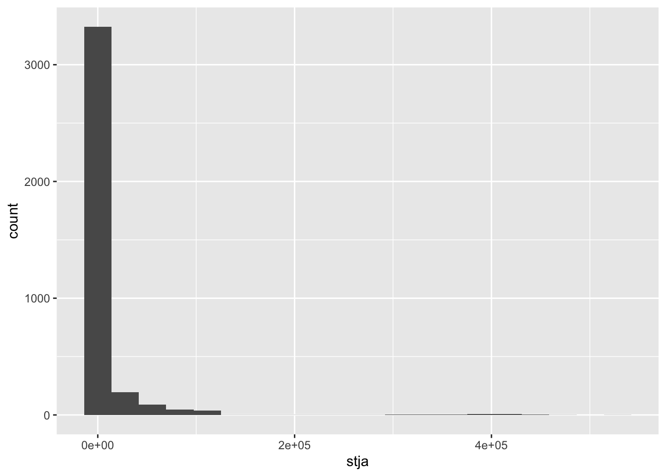
df_stja %>% filter(income != "Aggregates", stja >0) %>%
  ggplot(aes(stja)) + geom_histogram(bins = 20) + scale_x_log10()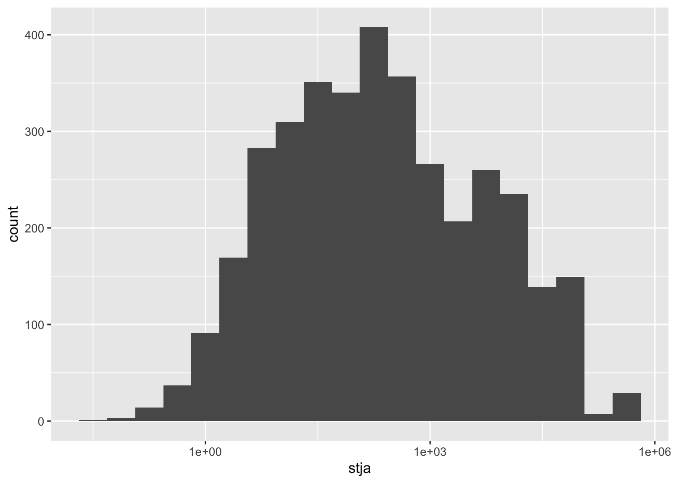
df_stja %>% filter(income != "Aggregates", income != "Not classified", stja >0) %>%
  ggplot(aes(stja, fill = income)) + geom_histogram(alpha = 0.7, bins = 20, color = "black") + scale_x_log10()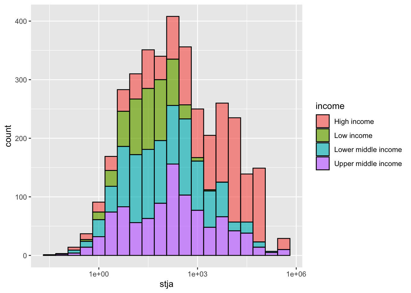
df_stja %>% filter(income != "Aggregates", income != "Not classified", stja >0) %>%
  ggplot(aes(stja, fill = income)) + geom_density(alpha = 0.3) + scale_x_log10()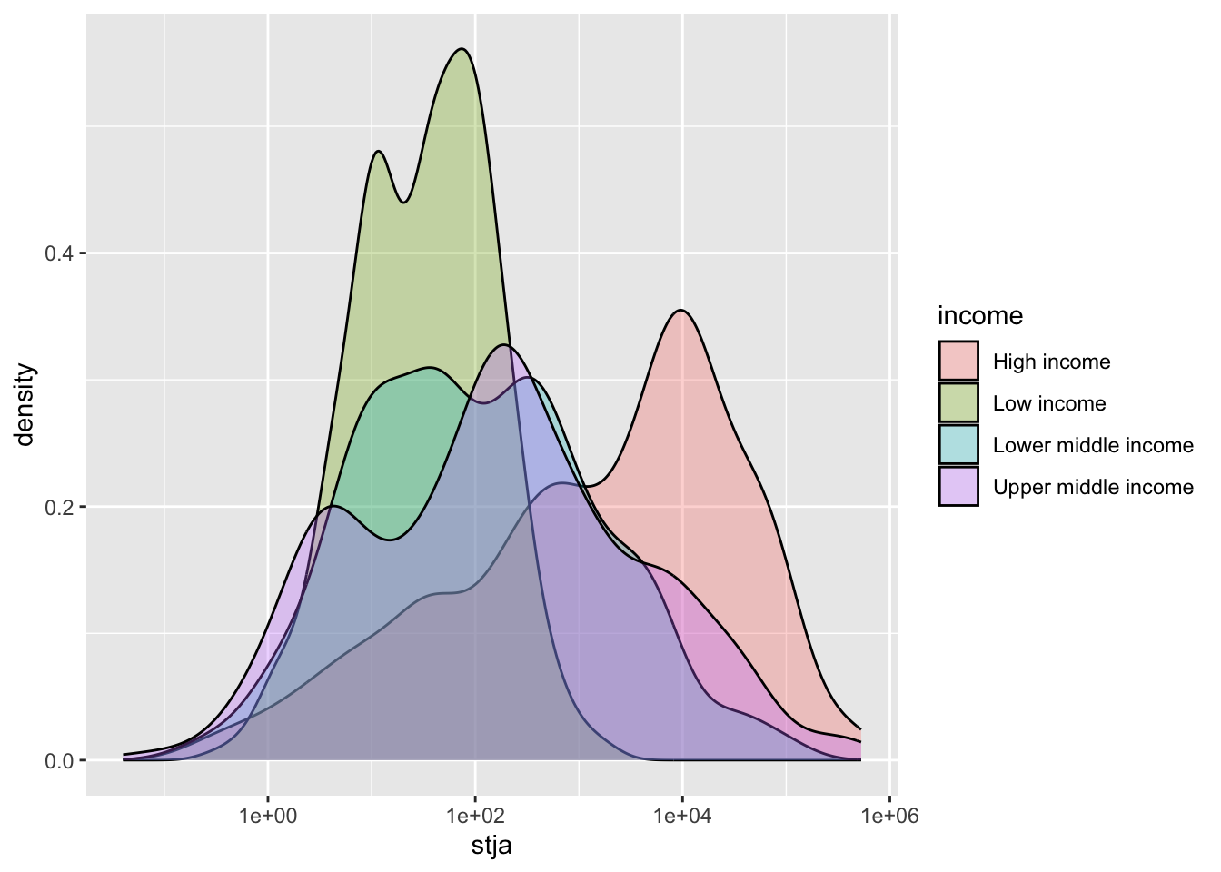
wdi_cache$series %>% filter(indicator == "MS.MIL.XPND.GD.ZS") %>% pull(name)
#> [1] "Military expenditure (% of GDP)"#> Rows: 9915 Columns: 13
#> ── Column specification ────────────────────────────────────
#> Delimiter: ","
#> chr (7): country, iso2c, iso3c, region, capital, income...
#> dbl (4): year, milxpnd, longitude, latitude
#> lgl (1): status
#> date (1): lastupdated
#>
#> ℹ Use `spec()` to retrieve the full column specification for this data.
#> ℹ Specify the column types or set `show_col_types = FALSE` to quiet this message.Default of the number of bins is 30. Here I chose binwidth = 0.5 (%).
df_milxpnd %>% filter(income != "Aggregates", year == 2021) %>%
  ggplot(aes(milxpnd, fill = income)) + geom_histogram(color = "black", binwidth = 0.5) +
  labs(title = "Military expenditure (% of GDP)")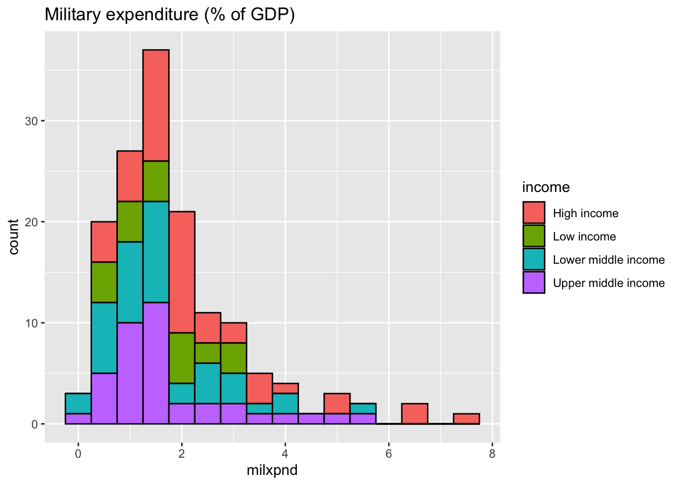
df_milxpnd %>% filter(income != "Aggregates", income != "Not classified", year == 2021) %>%
  ggplot(aes(milxpnd, fill = income)) + geom_density(binwidth = 0.5, alpha = 0.3) +
  labs(title = "Military expenditure (% of GDP)")
#> Warning in geom_density(binwidth = 0.5, alpha = 0.3):
#> Ignoring unknown parameters: `binwidth`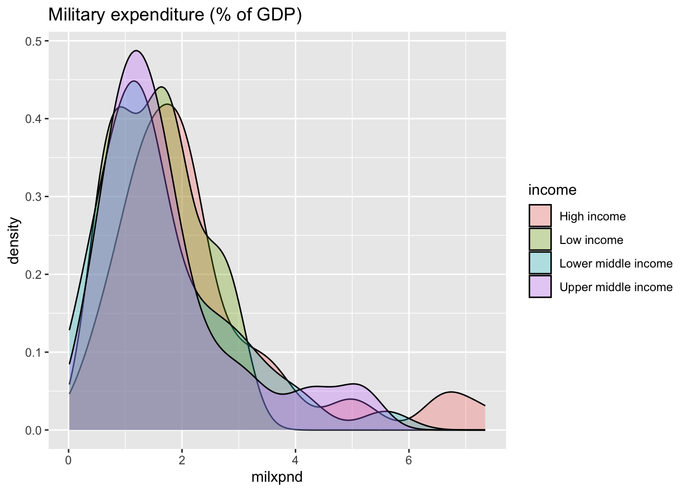
9.4.2 Q2. Effect of unemployed rate under pandemic depending on income groups
wdi_cache$series %>% filter(indicator == "SL.UEM.TOTL.ZS") %>% pull(name)
#> [1] "Unemployment, total (% of total labor force) (modeled ILO estimate)"#> Rows: 7285 Columns: 13
#> ── Column specification ────────────────────────────────────
#> Delimiter: ","
#> chr (7): country, iso2c, iso3c, region, capital, income...
#> dbl (4): year, ur, longitude, latitude
#> lgl (1): status
#> date (1): lastupdated
#>
#> ℹ Use `spec()` to retrieve the full column specification for this data.
#> ℹ Specify the column types or set `show_col_types = FALSE` to quiet this message.
df_ur %>% filter(income == "Aggregates") %>% filter(grepl('income', country)) %>%
  filter(year >= 2018) %>% ggplot() + geom_line(aes(x = year, y = ur, color = country))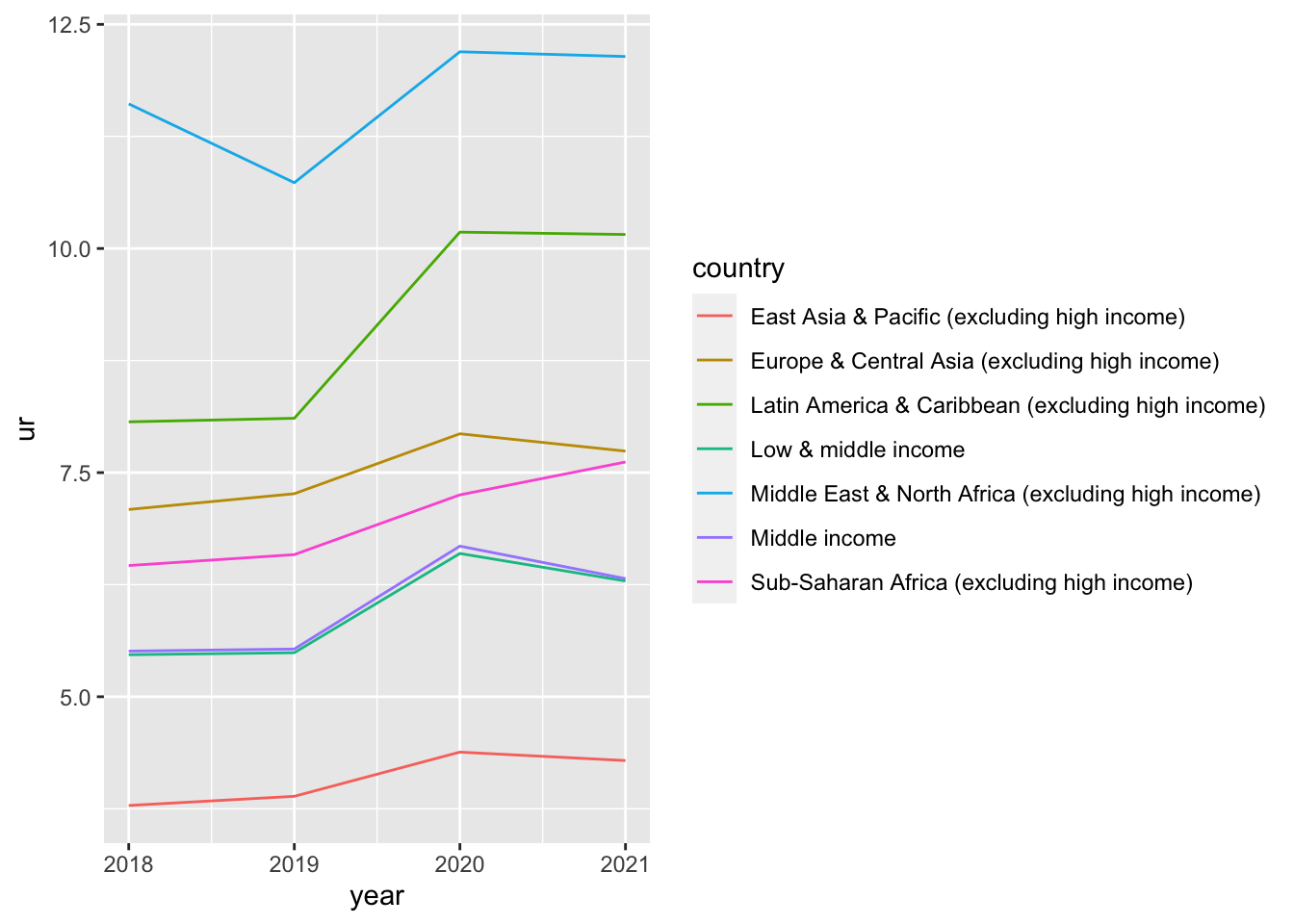
9.4.3 Q3. Add values at each data point.
wdi_cache$series %>% filter(indicator == "FP.CPI.TOTL.ZG") %>% pull(name)
#> [1] "Inflation, consumer prices (annual %)"
df_infl <- WDI(country = c("VN","CN","JP"),
               indicator = c(inf = "FP.CPI.TOTL.ZG"), extra = TRUE) %>% drop_na(inf)
#> Rows: 123 Columns: 13
#> ── Column specification ────────────────────────────────────
#> Delimiter: ","
#> chr (7): country, iso2c, iso3c, region, capital, income...
#> dbl (4): year, inf, longitude, latitude
#> lgl (1): status
#> date (1): lastupdated
#>
#> ℹ Use `spec()` to retrieve the full column specification for this data.
#> ℹ Specify the column types or set `show_col_types = FALSE` to quiet this message.
df_infl_s <- df_infl %>% filter(year %in% c(2000, 2005, 2010, 2015, 2020),
                   country %in% c("Japan", "Vietnam", "China"))
df_infl_s
#> # A tibble: 15 × 13
#>    country iso2c iso3c  year     inf status lastupdated
#>    <chr>   <chr> <chr> <dbl>   <dbl> <lgl>  <date>
#>  1 China   CN    CHN    2020  2.42   NA     2022-12-22
#>  2 China   CN    CHN    2015  1.44   NA     2022-12-22
#>  3 China   CN    CHN    2010  3.18   NA     2022-12-22
#>  4 China   CN    CHN    2005  1.78   NA     2022-12-22
#>  5 China   CN    CHN    2000  0.348  NA     2022-12-22
#>  6 Japan   JP    JPN    2020 -0.0250 NA     2022-12-22
#>  7 Japan   JP    JPN    2015  0.795  NA     2022-12-22
#>  8 Japan   JP    JPN    2010 -0.728  NA     2022-12-22
#>  9 Japan   JP    JPN    2005 -0.283  NA     2022-12-22
#> 10 Japan   JP    JPN    2000 -0.677  NA     2022-12-22
#> 11 Vietnam VN    VNM    2020  3.22   NA     2022-12-22
#> 12 Vietnam VN    VNM    2015  0.631  NA     2022-12-22
#> 13 Vietnam VN    VNM    2010  9.21   NA     2022-12-22
#> 14 Vietnam VN    VNM    2005  8.28   NA     2022-12-22
#> 15 Vietnam VN    VNM    2000 -1.71   NA     2022-12-22
#> # ℹ 6 more variables: region <chr>, capital <chr>,
#> #   longitude <dbl>, latitude <dbl>, income <chr>,
#> #   lending <chr>
df_infl_s %>%
  ggplot(aes(x = year, y = inf, color= country)) +
  geom_line() + geom_point() +
  geom_text(aes(label = round(inf,2)), nudge_y = 0.8) +
labs(title = "Inflation of Japan, Vietnam and China from 2000 to 2020",
     x = "", y = "Inflation, consumer prices (annual %)")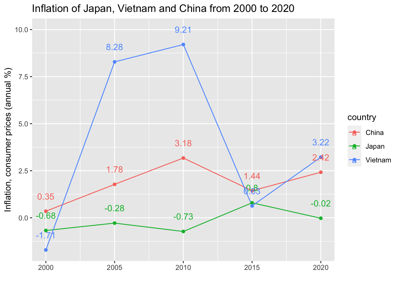
9.5 Regression Lines; Topic of EDA5
wdi_cache$series %>% filter(indicator %in% c("SI.POV.NAHC","SI.POV.MDIM")) %>% pull(name)
#> [1] "Multidimensional poverty headcount ratio (% of total population)"
#> [2] "Poverty headcount ratio at national poverty lines (% of population)"
df_wdi_poverty <- WDI(
  indicator = c(poverty = "SI.POV.NAHC", multipoverty = "SI.POV.MDIM", gdppercap = "NY.GDP.PCAP.KD"), start = 1990,
  extra = TRUE) %>% drop_na(poverty, multipoverty, gdppercap)
#> Rows: 292 Columns: 15
#> ── Column specification ────────────────────────────────────
#> Delimiter: ","
#> chr (7): country, iso2c, iso3c, region, capital, income...
#> dbl (6): year, poverty, multipoverty, gdppercap, longit...
#> lgl (1): status
#> date (1): lastupdated
#>
#> ℹ Use `spec()` to retrieve the full column specification for this data.
#> ℹ Specify the column types or set `show_col_types = FALSE` to quiet this message.
df_wdi_poverty %>%
  group_by(country, year) %>%
  mutate(mean_gdp = mean(gdppercap)) %>%
  mutate(mean_poverty= mean(poverty)) %>%
  ungroup() %>% filter(income != "Aggregates") %>%
  ggplot(aes(x = mean_gdp)) + geom_point(aes(y = mean_poverty, color = income)) +
  scale_x_log10() +  geom_smooth(aes(y = mean_poverty), formula = y~x, linetype="longdash", color = "black", method = "lm", se = FALSE) +
  labs(x = "GDP per capita", y = "poverty rate (% of population)", title = "Poverty rates and GDP per capita", subtitle="world countries, 1990-2021 average, by income level")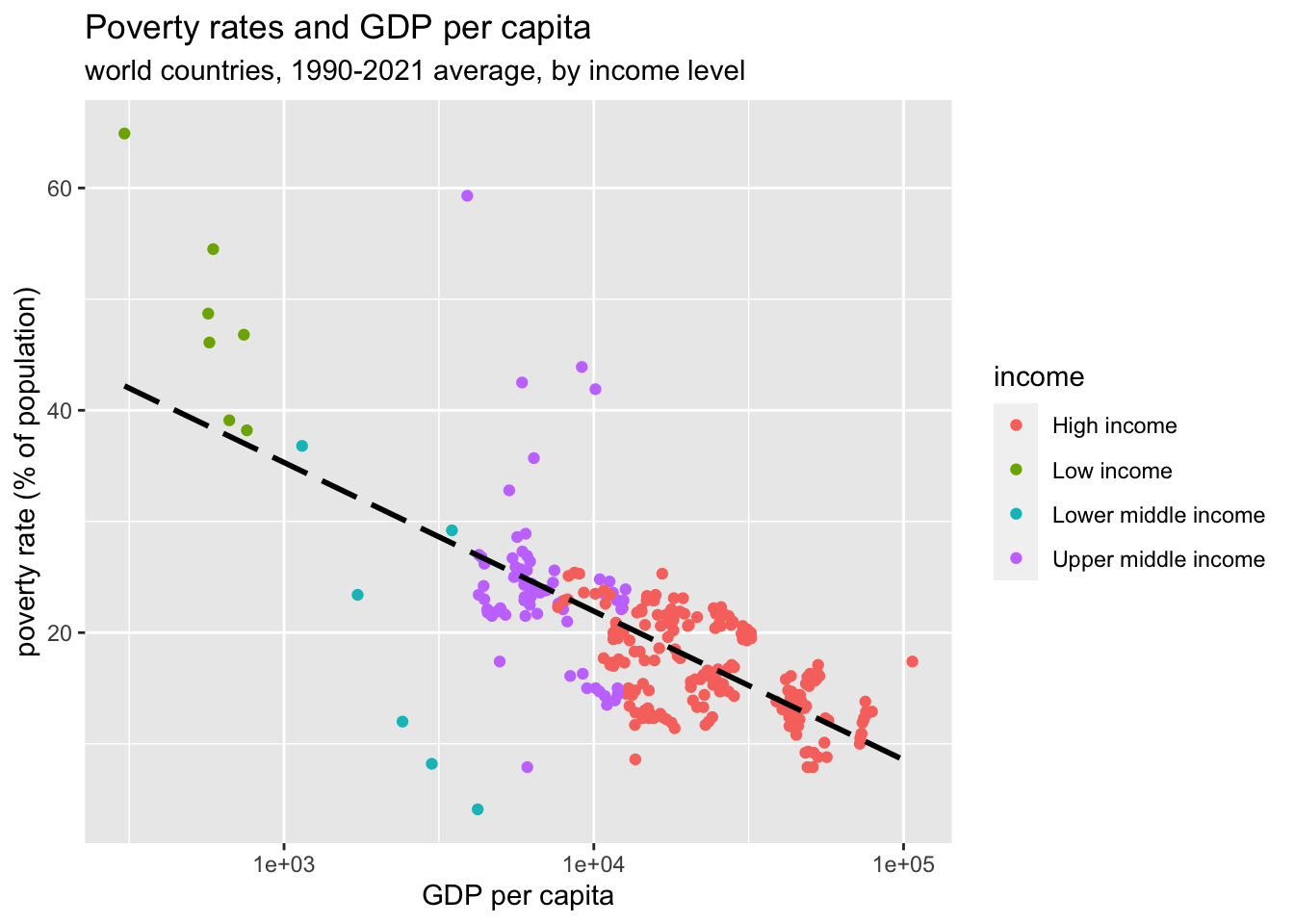
df_wdi_poverty %>%
  group_by(country, year) %>%
  mutate(mean_gdp = mean(gdppercap)) %>%
  mutate(mean_multipoverty= mean(multipoverty)) %>%
  ungroup() %>%
    filter(region !="Aggregates") %>% ggplot(aes(x = mean_gdp)) + geom_point(aes(y = mean_multipoverty, color = region)) +
  scale_x_log10() +
  geom_smooth(aes(y = mean_multipoverty), formula = y~x, linetype="longdash", color = "black", method = "lm", se = FALSE) + labs(x = "GDP per capita", y = "Multidimentinal poverty rate (% of population)", title = "Multidimentional Poverty rates and GDP per capita", subtitle="world countries, 1990-2021 average, by region")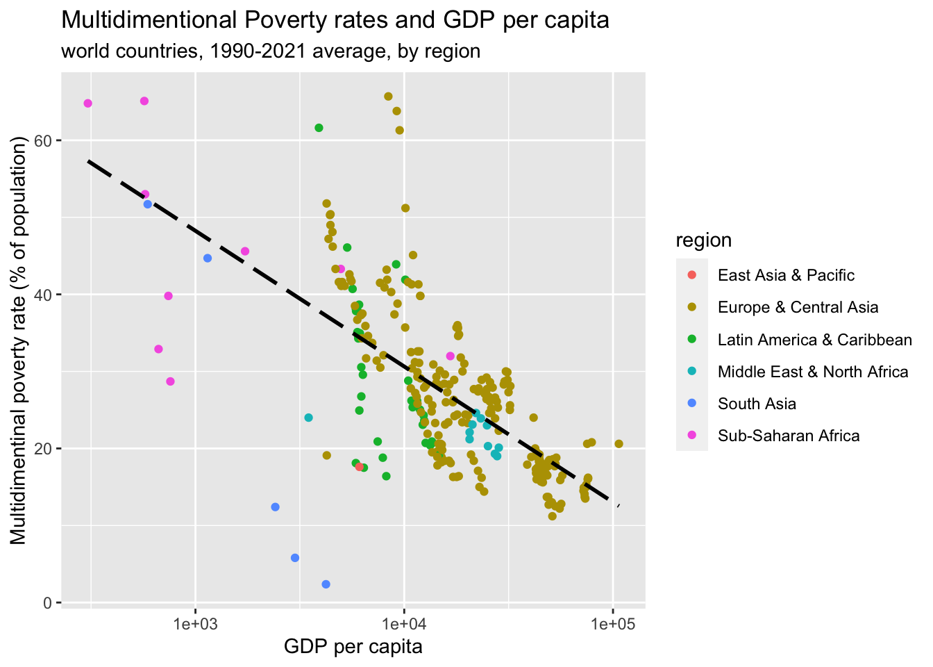
9.6 Appendix: A secondary axis
-
Specify a secondary axis
- This function is used in conjunction with a position scale to create a secondary axis, positioned opposite of the primary axis. All secondary axes must be based on a one-to-one transformation of the primary axes.
scale_y_continuous(sec.axis = sec_axis(~ . scaling_function))
9.6.1 Example
Suppose you have two indicators,
- NY.GDP.MKTP.KD: GDP (constant 2015 US$)
- NY.GDP.PCAP.KD: GDP per capita (constant 2015 US$)
WDIsearch(string = "NY.GDP.MKTP.KD", field = "indicator", short = FALSE, cache = wdi_cache)
#>               indicator
#> 12112    NY.GDP.MKTP.KD
#> 12113 NY.GDP.MKTP.KD.87
#> 12114 NY.GDP.MKTP.KD.ZG
#>                                           name
#> 12112                  GDP (constant 2015 US$)
#> 12113 GDP at market prices (constant 1987 US$)
#> 12114                    GDP growth (annual %)
#>                                                                                                                                                                                                                                                                                                                                                                                                                                                                                                                                                                                                                                                                                     description
#> 12112 GDP at purchaser's prices is the sum of gross value added by all resident producers in the economy plus any product taxes and minus any subsidies not included in the value of the products. It is calculated without making deductions for depreciation of fabricated assets or for depletion and degradation of natural resources. Data are in constant 2015 prices, expressed in U.S. dollars. Dollar figures for GDP are converted from domestic currencies using 2015 official exchange rates. For a few countries where the official exchange rate does not reflect the rate effectively applied to actual foreign exchange transactions, an alternative conversion factor is used.
#> 12113
#> 12114                                                                                                                                                                                                           Annual percentage growth rate of GDP at market prices based on constant local currency. Aggregates are based on constant 2015 prices, expressed in U.S. dollars. GDP is the sum of gross value added by all resident producers in the economy plus any product taxes and minus any subsidies not included in the value of the products. It is calculated without making deductions for depreciation of fabricated assets or for depletion and degradation of natural resources.
#>                     sourceDatabase
#> 12112 World Development Indicators
#> 12113        WDI Database Archives
#> 12114 World Development Indicators
#>                                                              sourceOrganization
#> 12112 World Bank national accounts data, and OECD National Accounts data files.
#> 12113
#> 12114 World Bank national accounts data, and OECD National Accounts data files.
WDIsearch(string = "NY.GDP.PCAP.KD", field = "indicator", short = FALSE, cache = wdi_cache)
#>               indicator                               name
#> 12127    NY.GDP.PCAP.KD GDP per capita (constant 2015 US$)
#> 12128 NY.GDP.PCAP.KD.ZG   GDP per capita growth (annual %)
#>                                                                                                                                                                                                                                                                                                                                                                                                                                                                                          description
#> 12127                                                                 GDP per capita is gross domestic product divided by midyear population. GDP is the sum of gross value added by all resident producers in the economy plus any product taxes and minus any subsidies not included in the value of the products. It is calculated without making deductions for depreciation of fabricated assets or for depletion and degradation of natural resources. Data are in constant 2015 U.S. dollars.
#> 12128 Annual percentage growth rate of GDP per capita based on constant local currency. GDP per capita is gross domestic product divided by midyear population. GDP at purchaser's prices is the sum of gross value added by all resident producers in the economy plus any product taxes and minus any subsidies not included in the value of the products. It is calculated without making deductions for depreciation of fabricated assets or for depletion and degradation of natural resources.
#>                     sourceDatabase
#> 12127 World Development Indicators
#> 12128 World Development Indicators
#>                                                              sourceOrganization
#> 12127 World Bank national accounts data, and OECD National Accounts data files.
#> 12128 World Bank national accounts data, and OECD National Accounts data files.
List the name of countries of ASEAN and BRICs using wdi_cache$country.
asean <- c("Brunei Darussalam", "Cambodia", "Lao PDR", "Myanmar",
           "Philippines", "Indonesia", "Malaysia", "Singapore")
brics <- c("Brazil", "Russian Federation", "India", "China")
Find the iso2c of the countries using wdi_cache$country.
wdi_cache$country %>%
  filter(country %in%
           c("Brunei Darussalam", "Cambodia", "Lao PDR", "Myanmar",
           "Philippines", "Indonesia", "Malaysia", "Singapore",
           "Brazil", "Russian Federation", "India", "China")) %>%
  pull(iso2c)
#>  [1] "BR" "BN" "CN" "ID" "IN" "KH" "LA" "MM" "MY" "PH" "RU"
#> [12] "SG"
Separate the iso3c’s of the countries with commas and read data using WDI.
wdi_gdp <- WDI(
  country = c("BR", "BN", "CN", "ID", "IN", "KH", "LA", "MM", "MY", "PH", "RU", "SG"),
  indicator = c(gdp = "NY.GDP.MKTP.KD", gdpPercap = "NY.GDP.PCAP.KD"),
  start = 1960, extra = TRUE, cache = wdi_cache)
#> Rows: 744 Columns: 14
#> ── Column specification ────────────────────────────────────
#> Delimiter: ","
#> chr (7): country, iso2c, iso3c, region, capital, income...
#> dbl (5): year, gdp, gdpPercap, longitude, latitude
#> lgl (1): status
#> date (1): lastupdated
#>
#> ℹ Use `spec()` to retrieve the full column specification for this data.
#> ℹ Specify the column types or set `show_col_types = FALSE` to quiet this message.
wdi_gdp %>% filter(country %in% asean) %>% drop_na(gdp, gdpPercap) %>% summary()
#>    country             iso2c              iso3c
#>  Length:424         Length:424         Length:424
#>  Class :character   Class :character   Class :character
#>  Mode  :character   Mode  :character   Mode  :character
#>
#>
#>
#>       year       status         lastupdated
#>  Min.   :1960   Mode:logical   Min.   :2022-12-22
#>  1st Qu.:1980   NA's:424       1st Qu.:2022-12-22
#>  Median :1995                  Median :2022-12-22
#>  Mean   :1994                  Mean   :2022-12-22
#>  3rd Qu.:2008                  3rd Qu.:2022-12-22
#>  Max.   :2021                  Max.   :2022-12-22
#>       gdp              gdpPercap          region
#>  Min.   :2.109e+09   Min.   :  144.0   Length:424
#>  1st Qu.:1.069e+10   1st Qu.:  978.2   Class :character
#>  Median :4.099e+10   Median : 1891.2   Mode  :character
#>  Mean   :1.149e+11   Mean   : 9718.5
#>  3rd Qu.:1.430e+11   3rd Qu.: 8777.6
#>  Max.   :1.066e+12   Max.   :66176.4
#>    capital            longitude         latitude
#>  Length:424         Min.   : 95.96   Min.   :-6.198
#>  Class :character   1st Qu.:101.68   1st Qu.: 1.289
#>  Mode  :character   Median :103.85   Median : 4.942
#>                     Mean   :106.52   Mean   : 8.035
#>                     3rd Qu.:114.95   3rd Qu.:14.552
#>                     Max.   :121.03   Max.   :21.914
#>     income            lending
#>  Length:424         Length:424
#>  Class :character   Class :character
#>  Mode  :character   Mode  :character
#>
#>
#>
Using the summary, decide the scaling of two variables, gdpPercap and gdp.
wdi_gdp %>% drop_na(gdp, gdpPercap) %>%
  filter(country %in% asean) %>%
  ggplot() +
  geom_line(aes(x = year, y = gdpPercap, linetype = country)) +
  geom_line(aes(x = year, y = gdp/(10^7), col = country)) +
  coord_trans(x ="identity", y="log10") +
  scale_y_continuous(sec.axis = sec_axis(~ . *(10^7), name = "gdp/(10^7)"))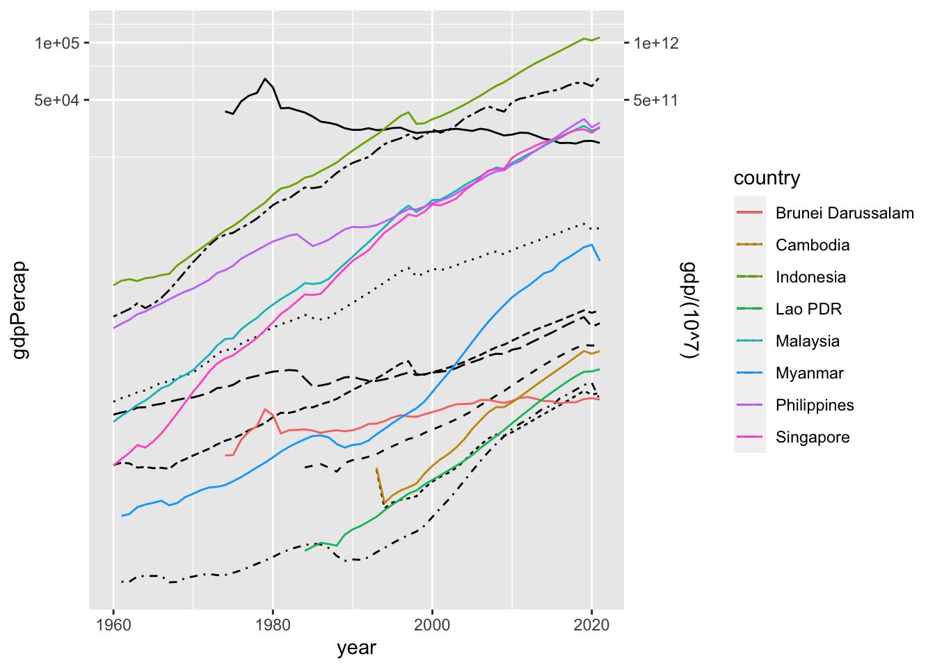
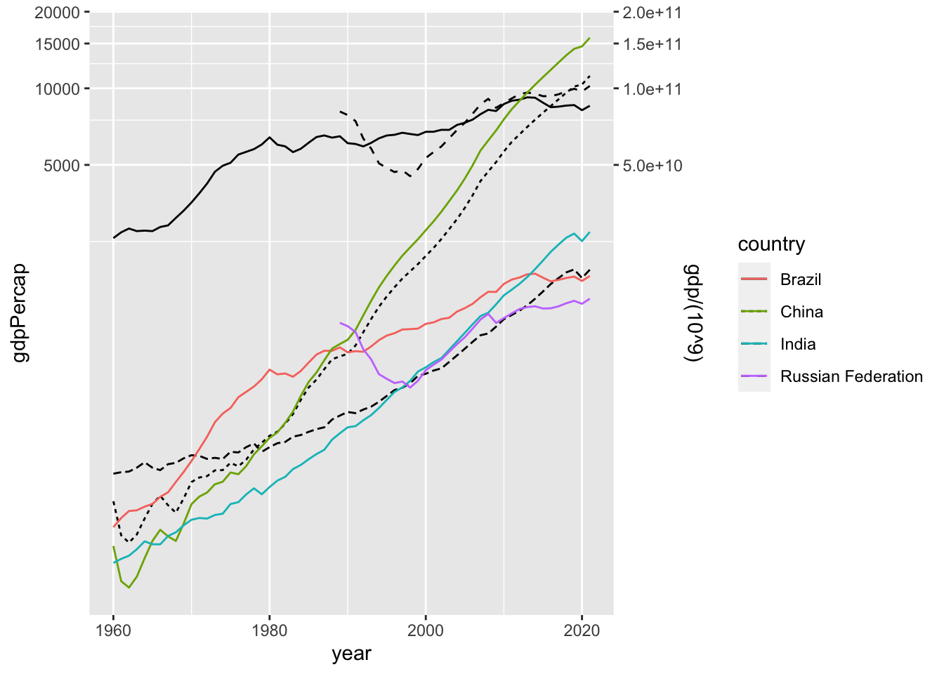
9.6.1.1 BRICs
wdi_gdp %>% filter(country %in% brics) %>% drop_na(gdp, gdpPercap) %>% summary()
#>    country             iso2c              iso3c
#>  Length:219         Length:219         Length:219
#>  Class :character   Class :character   Class :character
#>  Mode  :character   Mode  :character   Mode  :character
#>
#>
#>
#>       year       status         lastupdated
#>  Min.   :1960   Mode:logical   Min.   :2022-12-22
#>  1st Qu.:1978   NA's:219       1st Qu.:2022-12-22
#>  Median :1994                  Median :2022-12-22
#>  Mean   :1993                  Mean   :2022-12-22
#>  3rd Qu.:2008                  3rd Qu.:2022-12-22
#>  Max.   :2021                  Max.   :2022-12-22
#>       gdp              gdpPercap          region
#>  Min.   :1.091e+11   Min.   :  163.9   Length:219
#>  1st Qu.:3.564e+11   1st Qu.:  531.7   Class :character
#>  Median :9.215e+11   Median : 2758.9   Mode  :character
#>  Mean   :1.644e+12   Mean   : 3825.8
#>  3rd Qu.:1.500e+12   3rd Qu.: 6579.5
#>  Max.   :1.580e+13   Max.   :11188.3
#>    capital            longitude         latitude
#>  Length:219         Min.   :-47.93   Min.   :-15.78
#>  Class :character   1st Qu.:-47.93   1st Qu.:-15.78
#>  Mode  :character   Median : 77.22   Median : 28.64
#>                     Mean   : 46.88   Mean   : 23.38
#>                     3rd Qu.:116.29   3rd Qu.: 40.05
#>                     Max.   :116.29   Max.   : 55.76
#>     income            lending
#>  Length:219         Length:219
#>  Class :character   Class :character
#>  Mode  :character   Mode  :character
#>
#>
#>
Using the summary, decide the scaling of two variables, gdpPercap and gdp.
wdi_gdp %>% drop_na(gdp, gdpPercap) %>%
  filter(country %in% brics) %>%
  ggplot() +
  geom_line(aes(x = year, y = gdpPercap, linetype = country)) +
  geom_line(aes(x = year, y = gdp/(10^9), col = country)) +
  coord_trans(x ="identity", y="log10") +
  scale_y_continuous(sec.axis = sec_axis(~ . *(10^7), name = "gdp/(10^9)"))