Chapter 7 Topics in Exploratory Data Analysis I　

Prof. Taisei Kaizoji and R Notebook Compiled by HS

Get AGCO2rv.csv from Moodle and place it at the same place as this file.
Reference: Data Analysis for Researchers Week 7(02/02)
- Inference Statistics Regression Analysis

Summary

Give a descriptive name to each variable, when importing data by WDI command.
Save data of investigation by write_csv, but if you have RNotebook, you do not need to save at every step.
If you use pipe in tidyverse, i.e, %>%, properly, you do not need to attach(data) or dettach(data).

Dot Place Holder in `lm`.

In the following, the following format is used.

df %>% lm(y ~ x, .)

This is same as

lm(y ~ x, data = df)

‘.’ is called the dot place holder. Recall that most of the function (or command) we use in tidyverse, the first argument is the data frame. When we use piping, we omit the first argiment. For example,

df %>% ggplot(aes(x, y)) + geom_point()

is same as

ggplot(df, aes(x,y)) + geom_point()

However, the data frame argument of lm() is not the first one, therefore we use the dot place holder to show the place the data frame should be inserted.

7.1 Part I: Regression 1:

Run the following only once, or you can install these packages using install packages in the Tool menu.

install.packages("car")
install.packages("modelsummary")

7.1.1 Why does GDP vary from country to country?

library(tidyverse) # tidyverse Package, a collection of packages for data science
library(WDI) # WDI Package for World Development Indicators
library(car) #VIF Tool for checking multi-collinearity

##  要求されたパッケージ carData をロード中です

## 
##  次のパッケージを付け加えます: 'car'

##  以下のオブジェクトは 'package:dplyr' からマスクされています:
## 
##     recode

##  以下のオブジェクトは 'package:purrr' からマスクされています:
## 
##     some

library(modelsummary) # Tool for writting tables of the regression results

WDI Indicators
- NY.GDP.MKTP.CD: GDP (current US$)
- SP.POP.TOTL: Population, total
- AG.LND.TOTL.K2: Land area (sq. km)

wb <- as_tibble(WDI(country="all", 
                    indicator=c(gdp = "NY.GDP.MKTP.CD", pop = "SP.POP.TOTL", land = "AG.LND.TOTL.K2"),
                    start=1960, end=2020,
                    extra=TRUE))
wb

## # A tibble: 16,226 × 15
##    country     iso2c iso3c  year status lastupda…¹      gdp    pop   land region
##    <chr>       <chr> <chr> <int> <chr>  <chr>         <dbl>  <dbl>  <dbl> <chr> 
##  1 Afghanistan AF    AFG    2020 ""     2022-09-16  2.01e10 3.89e7 652230 South…
##  2 Afghanistan AF    AFG    2019 ""     2022-09-16  1.88e10 3.80e7 652230 South…
##  3 Afghanistan AF    AFG    2017 ""     2022-09-16  1.88e10 3.63e7 652230 South…
##  4 Afghanistan AF    AFG    1993 ""     2022-09-16 NA       1.58e7 652230 South…
##  5 Afghanistan AF    AFG    1983 ""     2022-09-16 NA       1.25e7 652230 South…
##  6 Afghanistan AF    AFG    2006 ""     2022-09-16  6.97e 9 2.64e7 652230 South…
##  7 Afghanistan AF    AFG    2018 ""     2022-09-16  1.81e10 3.72e7 652230 South…
##  8 Afghanistan AF    AFG    1981 ""     2022-09-16  3.48e 9 1.32e7 652230 South…
##  9 Afghanistan AF    AFG    2016 ""     2022-09-16  1.81e10 3.54e7 652230 South…
## 10 Afghanistan AF    AFG    1989 ""     2022-09-16 NA       1.19e7 652230 South…
## # … with 16,216 more rows, 5 more variables: capital <chr>, longitude <chr>,
## #   latitude <chr>, income <chr>, lending <chr>, and abbreviated variable name
## #   ¹lastupdated

wb_ag20 <- wb %>% filter(year == 2020 & region=="Aggregates")
wb_ag20

## # A tibble: 42 × 15
##    country iso2c iso3c  year status lastu…¹     gdp    pop   land region capital
##    <chr>   <chr> <chr> <int> <chr>  <chr>     <dbl>  <dbl>  <dbl> <chr>  <chr>  
##  1 Africa… ZH    AFE    2020 ""     2022-0… 9.22e11 6.77e8 1.48e7 Aggre… ""     
##  2 Africa… ZI    AFW    2020 ""     2022-0… 7.84e11 4.59e8 9.05e6 Aggre… ""     
##  3 Arab W… 1A    ARB    2020 ""     2022-0… 2.50e12 4.36e8 1.31e7 Aggre… ""     
##  4 Caribb… S3    CSS    2020 ""     2022-0… 6.59e10 7.44e6 4.05e5 Aggre… ""     
##  5 Centra… B8    CEB    2020 ""     2022-0… 1.65e12 1.02e8 1.11e6 Aggre… ""     
##  6 Early-… V2    EAR    2020 ""     2022-0… 1.08e13 3.33e9 3.33e7 Aggre… ""     
##  7 East A… Z4    EAS    2020 ""     2022-0… 2.71e13 2.36e9 2.45e7 Aggre… ""     
##  8 East A… 4E    EAP    2020 ""     2022-0… 1.75e13 2.11e9 1.60e7 Aggre… ""     
##  9 East A… T4    TEA    2020 ""     2022-0… 1.75e13 2.09e9 1.59e7 Aggre… ""     
## 10 Euro a… XC    EMU    2020 ""     2022-0… 1.30e13 3.43e8 2.68e6 Aggre… ""     
## # … with 32 more rows, 4 more variables: longitude <chr>, latitude <chr>,
## #   income <chr>, lending <chr>, and abbreviated variable name ¹lastupdated

7.1.2 Regression

wb_ag20 %>% ggplot(aes(pop, gdp)) +
  geom_point() +
  geom_smooth(method = "lm", se = FALSE) +
  labs(title = "GDP and Population", 
       x = "total population", y = "GDP")

## `geom_smooth()` using formula = 'y ~ x'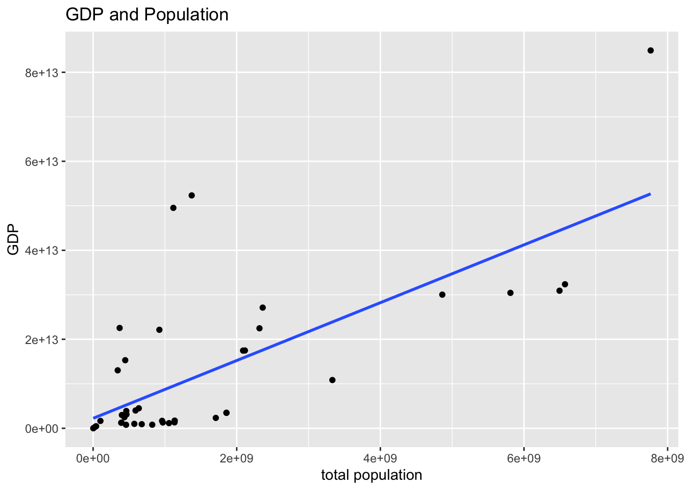

gdp_pop <-wb_ag20 %>% lm(gdp ~ pop, .)
summary(gdp_pop)

## 
## Call:
## lm(formula = gdp ~ pop, data = .)
## 
## Residuals:
##        Min         1Q     Median         3Q        Max 
## -1.352e+13 -7.740e+12 -2.406e+12  8.240e+11  4.118e+13 
## 
## Coefficients:
##              Estimate Std. Error t value Pr(>|t|)    
## (Intercept) 2.234e+12  2.591e+12   0.862    0.394    
## pop         6.498e+03  1.044e+03   6.224 2.29e-07 ***
## ---
## Signif. codes:  0 '***' 0.001 '**' 0.01 '*' 0.05 '.' 0.1 ' ' 1
## 
## Residual standard error: 1.291e+13 on 40 degrees of freedom
## Multiple R-squared:  0.492,  Adjusted R-squared:  0.4793 
## F-statistic: 38.73 on 1 and 40 DF,  p-value: 2.291e-07

wb_ag20 %>% ggplot(aes(land, gdp)) +
  geom_point() +
  geom_smooth(method = "lm", se = FALSE) +
  labs(title = "GDP and Land Area", 
       x = "land area", y = "GDP")

## `geom_smooth()` using formula = 'y ~ x'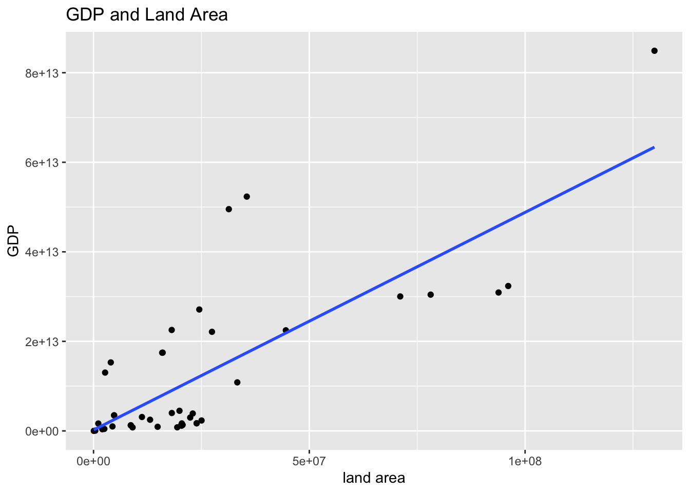

gdp_land <-wb_ag20 %>% lm(gdp ~ land, .)
summary(gdp_land)

## 
## Call:
## lm(formula = gdp ~ land, data = .)
## 
## Residuals:
##        Min         1Q     Median         3Q        Max 
## -1.491e+13 -8.021e+12 -3.149e+12  9.542e+11  3.487e+13 
## 
## Coefficients:
##              Estimate Std. Error t value Pr(>|t|)    
## (Intercept) 2.100e+11  2.402e+12   0.087    0.931    
## land        4.860e+05  6.353e+04   7.649 2.38e-09 ***
## ---
## Signif. codes:  0 '***' 0.001 '**' 0.01 '*' 0.05 '.' 0.1 ' ' 1
## 
## Residual standard error: 1.154e+13 on 40 degrees of freedom
## Multiple R-squared:  0.594,  Adjusted R-squared:  0.5838 
## F-statistic: 58.51 on 1 and 40 DF,  p-value: 2.376e-09

gdp_pop_and_land <-wb_ag20 %>% lm(gdp ~ pop + land, .)
summary(gdp_pop_and_land)

## 
## Call:
## lm(formula = gdp ~ pop + land, data = .)
## 
## Residuals:
##        Min         1Q     Median         3Q        Max 
## -1.397e+13 -9.135e+12 -3.362e+12  3.760e+12  3.334e+13 
## 
## Coefficients:
##               Estimate Std. Error t value Pr(>|t|)   
## (Intercept)  1.464e+11  2.422e+12   0.060  0.95209   
## pop         -1.767e+03  2.740e+03  -0.645  0.52270   
## land         5.990e+05  1.865e+05   3.212  0.00264 **
## ---
## Signif. codes:  0 '***' 0.001 '**' 0.01 '*' 0.05 '.' 0.1 ' ' 1
## 
## Residual standard error: 1.163e+13 on 39 degrees of freedom
## Multiple R-squared:  0.5982, Adjusted R-squared:  0.5776 
## F-statistic: 29.04 on 2 and 39 DF,  p-value: 1.893e-08

gpa_models <- list(gdp_pop = gdp_pop, gdp_land = gdp_land, gdp_pop_and_land = gdp_pop_and_land)
msummary(gpa_models, statistic = 'p.value')

	gdp_pop	gdp_land	gdp_pop_and_land
(Intercept)	2e+12	2e+11	1e+11
	(0.394)	(0.931)	(0.952)
pop	6498.247		-1767.039
	(<0.001)		(0.523)
land		486003.841	598971.604
		(<0.001)	(0.003)
Num.Obs.	42	42	42
R2	0.492	0.594	0.598
R2 Adj.	0.479	0.584	0.578
AIC	2659.0	2649.6	2651.2
BIC	2664.3	2654.8	2658.1
Log.Lik.	-1326.519	-1321.813	-1321.590
RMSE	1e+13	1e+13	1e+13

The default is: msummary(gpa_models). msummary(gpa_models, statistic = 'p.value') replaces the standard error by p-value. Compare the following with the one above and the Std.Error of the summaries of each model.

msummary(gpa_models)

	gdp_pop	gdp_land	gdp_pop_and_land
(Intercept)	2e+12	2e+11	1e+11
	(3e+12)	(2e+12)	(2e+12)
pop	6498.247		-1767.039
	(1044.119)		(2739.542)
land		486003.841	598971.604
		(63534.820)	(186468.820)
Num.Obs.	42	42	42
R2	0.492	0.594	0.598
R2 Adj.	0.479	0.584	0.578
AIC	2659.0	2649.6	2651.2
BIC	2664.3	2654.8	2658.1
Log.Lik.	-1326.519	-1321.813	-1321.590
RMSE	1e+13	1e+13	1e+13

wb_ag20 %>% ggplot(aes(pop, land)) +
  geom_point() +
  geom_smooth(method = "lm", se = FALSE) +
  labs(title = "population and Land", 
       x = "population", y = "land")

## `geom_smooth()` using formula = 'y ~ x'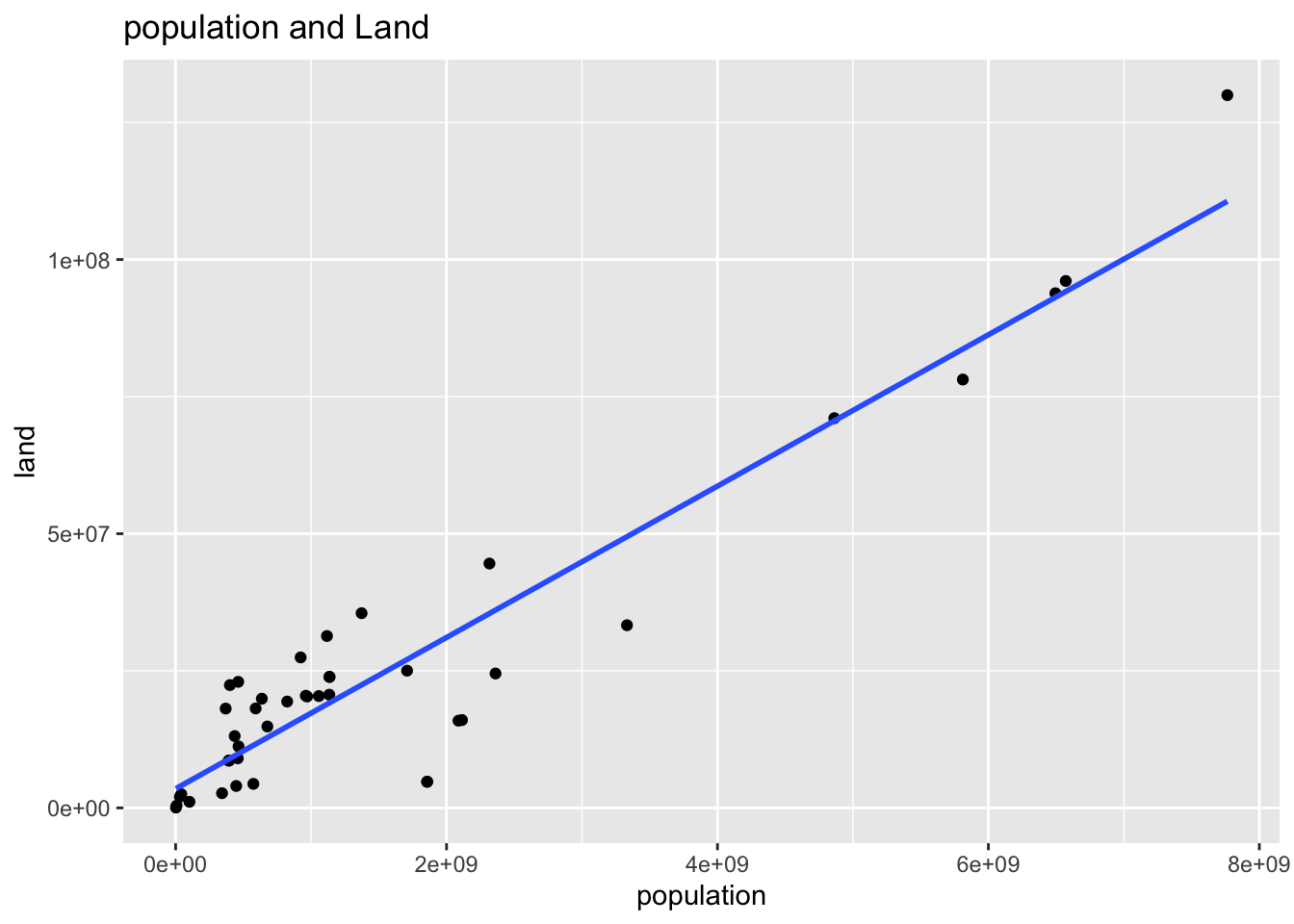

7.1.3 Checking for multicollinearity

pop_land <-wb_ag20 %>% lm(pop ~ land, .)
summary(pop_land)

## 
## Call:
## lm(formula = pop ~ land, data = .)
## 
## Residuals:
##        Min         1Q     Median         3Q        Max 
## -994986967 -376750174 -122152277  304321331 1587865293 
## 
## Coefficients:
##               Estimate Std. Error t value Pr(>|t|)    
## (Intercept) -3.594e+07  1.397e+08  -0.257    0.798    
## land         6.393e+01  3.694e+00  17.307   <2e-16 ***
## ---
## Signif. codes:  0 '***' 0.001 '**' 0.01 '*' 0.05 '.' 0.1 ' ' 1
## 
## Residual standard error: 671200000 on 40 degrees of freedom
## Multiple R-squared:  0.8822, Adjusted R-squared:  0.8792 
## F-statistic: 299.5 on 1 and 40 DF,  p-value: < 2.2e-16

7.1.4 vif: Determination of multi-collinearity

VIF = 1/(1-{R_i}²)

7.1.4.1 VIF (Variance Inflation Factor)

gdp_pop_and_land %>% vif()

##      pop     land 
## 8.487931 8.487931

7.1.4.2 Conclusion

Regions which have large population have large GDP.
It was also found that the larger the region, the more populated the region. This suggests that the GPs of regions with large regions and large populations are significant.
This result suggests a positive relationship between population and economic activity.

7.2 A time series data of World from 1960 to 2020

wb_world <- wb %>% filter(country=="World") %>% arrange(year)
wb_world

## # A tibble: 61 × 15
##    country iso2c iso3c  year status lastupdated     gdp       pop    land region
##    <chr>   <chr> <chr> <int> <chr>  <chr>         <dbl>     <dbl>   <dbl> <chr> 
##  1 World   1W    WLD    1960 ""     2022-09-16  1.39e12    3.03e9 NA      Aggre…
##  2 World   1W    WLD    1961 ""     2022-09-16  1.45e12    3.07e9  1.30e8 Aggre…
##  3 World   1W    WLD    1962 ""     2022-09-16  1.55e12    3.12e9  1.30e8 Aggre…
##  4 World   1W    WLD    1963 ""     2022-09-16  1.67e12    3.19e9  1.30e8 Aggre…
##  5 World   1W    WLD    1964 ""     2022-09-16  1.83e12    3.26e9  1.30e8 Aggre…
##  6 World   1W    WLD    1965 ""     2022-09-16  1.99e12    3.32e9  1.30e8 Aggre…
##  7 World   1W    WLD    1966 ""     2022-09-16  2.16e12    3.39e9  1.30e8 Aggre…
##  8 World   1W    WLD    1967 ""     2022-09-16  2.30e12    3.46e9  1.30e8 Aggre…
##  9 World   1W    WLD    1968 ""     2022-09-16  2.48e12    3.53e9  1.30e8 Aggre…
## 10 World   1W    WLD    1969 ""     2022-09-16  2.74e12    3.61e9  1.30e8 Aggre…
## # … with 51 more rows, and 5 more variables: capital <chr>, longitude <chr>,
## #   latitude <chr>, income <chr>, lending <chr>

wb_world %>% ggplot() + 
  geom_line(aes(x = year, y = gdp)) +
  labs(title = "GDP (current US$)")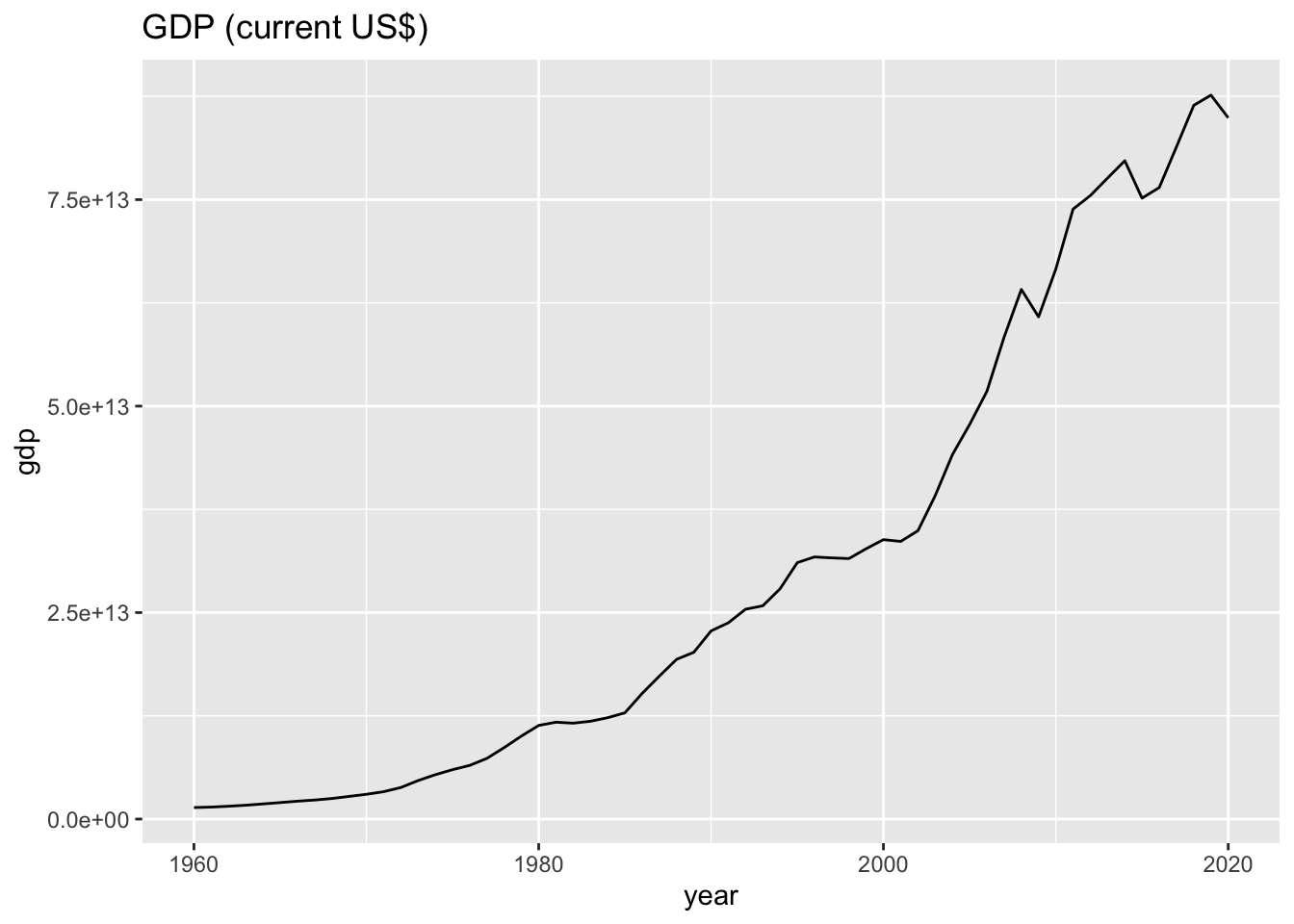

wb_world %>% ggplot() + 
  geom_line(aes(x = year, y = pop)) +
  labs(title = "Total population)")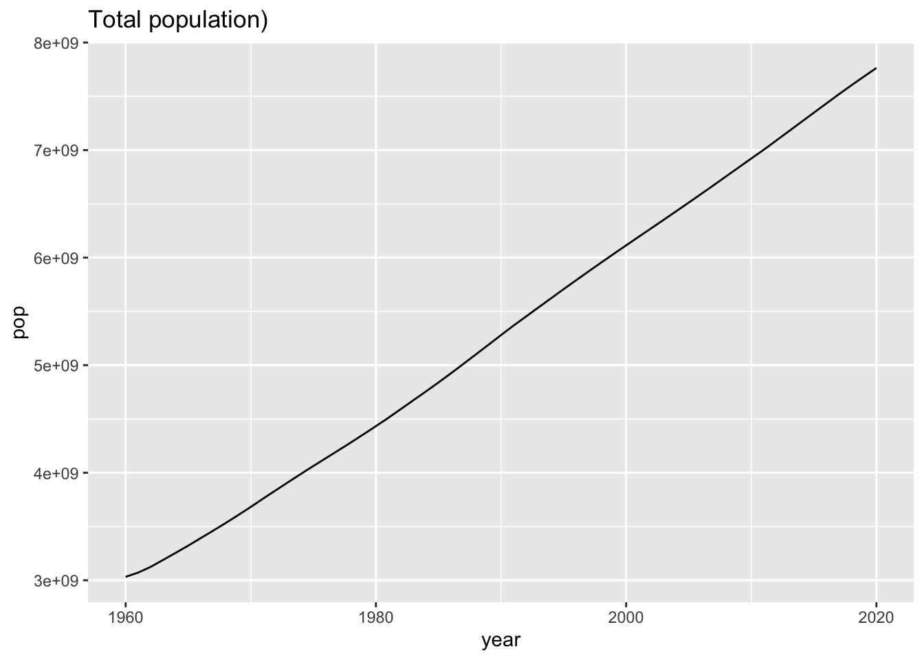

wb_world %>% lm(gdp ~ pop, .) %>% summary()

## 
## Call:
## lm(formula = gdp ~ pop, data = .)
## 
## Residuals:
##        Min         1Q     Median         3Q        Max 
## -1.334e+13 -7.513e+12 -1.944e+12  6.913e+12  1.350e+13 
## 
## Coefficients:
##               Estimate Std. Error t value Pr(>|t|)    
## (Intercept) -6.857e+13  4.151e+12  -16.52   <2e-16 ***
## pop          1.862e+04  7.563e+02   24.63   <2e-16 ***
## ---
## Signif. codes:  0 '***' 0.001 '**' 0.01 '*' 0.05 '.' 0.1 ' ' 1
## 
## Residual standard error: 8.396e+12 on 59 degrees of freedom
## Multiple R-squared:  0.9113, Adjusted R-squared:  0.9098 
## F-statistic: 606.4 on 1 and 59 DF,  p-value: < 2.2e-16

wb_world %>% ggplot() +
  geom_point(aes(pop, gdp)) +
  labs(title = "World GDP and World population", 
       x = "Total population", y = "GDP (current US$)")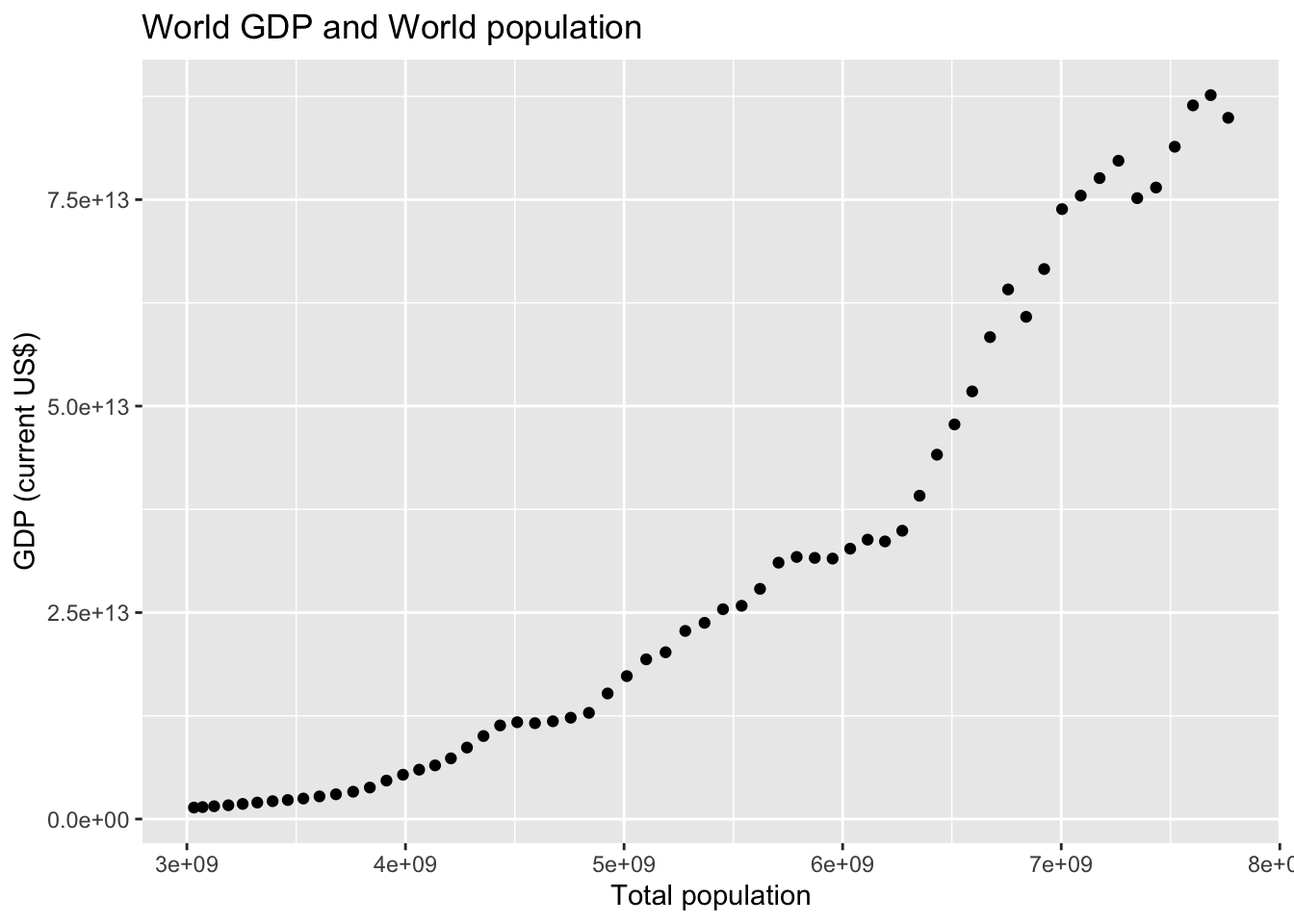

wb_world_extra <- wb_world %>% mutate(diff_gdp = gdp - lag(gdp), diff_pop = pop - lag(pop)) 
wb_world_extra

## # A tibble: 61 × 17
##    country iso2c iso3c  year status lastupdated     gdp       pop    land region
##    <chr>   <chr> <chr> <int> <chr>  <chr>         <dbl>     <dbl>   <dbl> <chr> 
##  1 World   1W    WLD    1960 ""     2022-09-16  1.39e12    3.03e9 NA      Aggre…
##  2 World   1W    WLD    1961 ""     2022-09-16  1.45e12    3.07e9  1.30e8 Aggre…
##  3 World   1W    WLD    1962 ""     2022-09-16  1.55e12    3.12e9  1.30e8 Aggre…
##  4 World   1W    WLD    1963 ""     2022-09-16  1.67e12    3.19e9  1.30e8 Aggre…
##  5 World   1W    WLD    1964 ""     2022-09-16  1.83e12    3.26e9  1.30e8 Aggre…
##  6 World   1W    WLD    1965 ""     2022-09-16  1.99e12    3.32e9  1.30e8 Aggre…
##  7 World   1W    WLD    1966 ""     2022-09-16  2.16e12    3.39e9  1.30e8 Aggre…
##  8 World   1W    WLD    1967 ""     2022-09-16  2.30e12    3.46e9  1.30e8 Aggre…
##  9 World   1W    WLD    1968 ""     2022-09-16  2.48e12    3.53e9  1.30e8 Aggre…
## 10 World   1W    WLD    1969 ""     2022-09-16  2.74e12    3.61e9  1.30e8 Aggre…
## # … with 51 more rows, and 7 more variables: capital <chr>, longitude <chr>,
## #   latitude <chr>, income <chr>, lending <chr>, diff_gdp <dbl>, diff_pop <dbl>

wb_world_extra %>% ggplot(aes(x = year, y = diff_gdp)) + geom_line() +
  labs(title = "World GDP changes", y = "gdp changes")

## Warning: Removed 1 row containing missing values (`geom_line()`).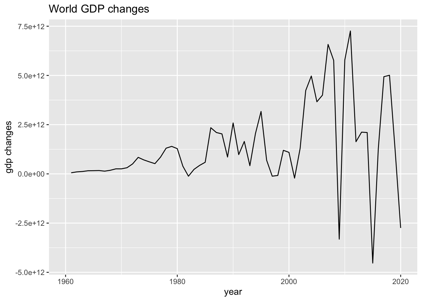

wb_world_extra %>% ggplot(aes(x = year, y = diff_pop)) + geom_line() +
  labs(title = "World population changes", y = "population changes")

## Warning: Removed 1 row containing missing values (`geom_line()`).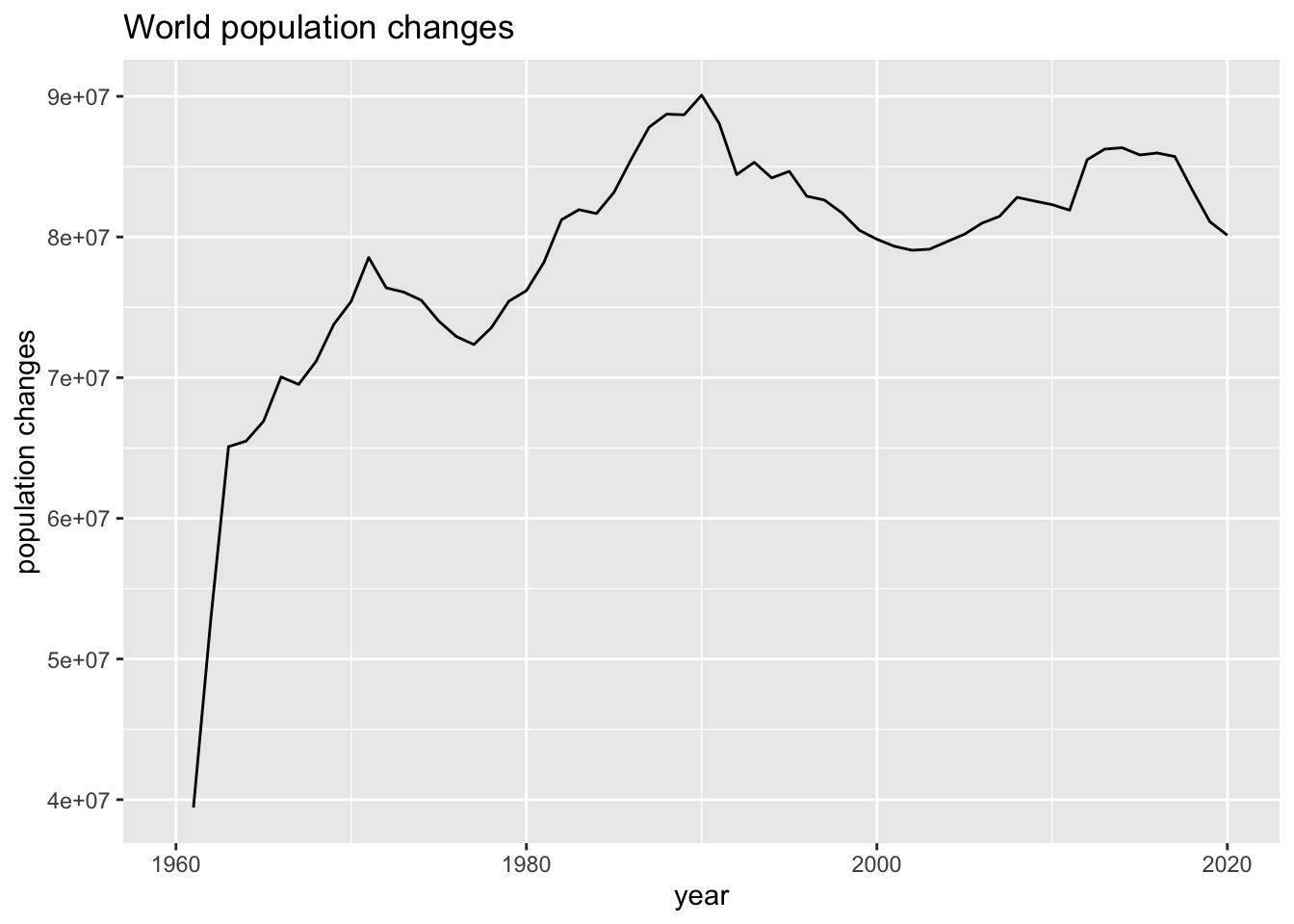

wb_world_extra %>% ggplot(aes(x = diff_pop, y = diff_gdp)) + geom_point() +
  geom_smooth(method = "lm", se = FALSE) + 
  labs(title = "World GDP changes and World GDP changes", x = "population changes", y = "GDP changes")

## `geom_smooth()` using formula = 'y ~ x'

## Warning: Removed 1 rows containing non-finite values (`stat_smooth()`).

## Warning: Removed 1 rows containing missing values (`geom_point()`).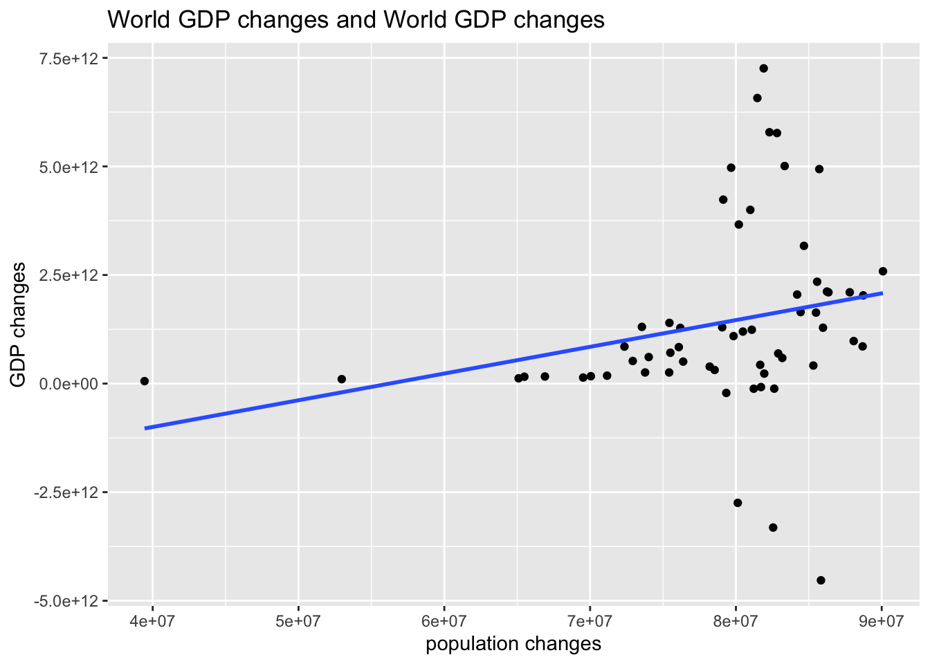

wb_world_extra %>% lm(diff_gdp ~ diff_pop, .) %>% summary()

## 
## Call:
## lm(formula = diff_gdp ~ diff_pop, data = .)
## 
## Residuals:
##        Min         1Q     Median         3Q        Max 
## -6.350e+12 -9.506e+11 -3.699e+11  3.100e+11  5.679e+12 
## 
## Coefficients:
##               Estimate Std. Error t value Pr(>|t|)  
## (Intercept) -3.460e+12  2.553e+12  -1.355   0.1806  
## diff_pop     6.152e+04  3.219e+04   1.911   0.0609 .
## ---
## Signif. codes:  0 '***' 0.001 '**' 0.01 '*' 0.05 '.' 0.1 ' ' 1
## 
## Residual standard error: 2.114e+12 on 58 degrees of freedom
##   ( 1 個の観測値が欠損のため削除されました )
## Multiple R-squared:  0.05925,    Adjusted R-squared:  0.04303 
## F-statistic: 3.653 on 1 and 58 DF,  p-value: 0.06092

7.2.1 Excercise:

Select a region from the following;

East Asia & Pacific
Europe & Central Asia
Middle East & North Africa
Sub-Saharan Africa
Latin America & Caribbean

Preform regression analysis.
Select the best model.

7.3 Regression 2 : CO2 Emission

7.3.1 Project

Problem: “What are the causes of increased CO2 emissions?”
Plan: To develop and test the hypothesis that CO2 emissions depends on GDP, population and land under cereal production of each region.
Data: Using the World Bank’s World Development Indicators (WDI), we will collect data on GDP, population and land area for regions around the world.
- WDIindicators
- GDP(Y):“NY.GDP.MKTP.CD”
- Total Population (X1): “SP.POP.TOTL”
- Land under cereal production (hectares): “AG.LND.CREL.HA”

7.3.1.1 Regression Analysis

Regression equation:Y =c + a x1 + b x2 + d x3 Y: CO2 emission: independent variable
- x1: GDP (Y) : independent variable
- x2: Total Population (X1) : independent variable x3: Land under cereal production (hectares): independent variable
We perform a regression analysis of the above regression equation (estimate the parameters, c (intercept), a, b, d) and elect the best model.

7.3.1.2 WDI Indicator cordes

co2 = EN.ATM.CO2E.KT: CO2 Emission
gdp = NY.GDP.MKTP.CD: GDP (current USD)
pop = SP.POP.TOTL: Total Population
cereal = AG.LND.CREL.HA: Land under cereal production (hectares)

WDIsearch(string = "EN.ATM.CO2E.KT", field = "indicator", short = FALSE)[[3]]

## [1] "Carbon dioxide emissions are those stemming from the burning of fossil fuels and the manufacture of cement. They include carbon dioxide produced during consumption of solid, liquid, and gas fuels and gas flaring."

wb_co2<- as_tibble(WDI(country="all", 
                   indicator=c(co2 = "EN.ATM.CO2E.KT",
                               gdp = "NY.GDP.MKTP.CD",
                               pop = "SP.POP.TOTL",
                               cereal = "AG.LND.CREL.HA"),
                   start=1960,
                   end=2020,
                   extra=TRUE))
wb_co2

## # A tibble: 16,226 × 16
##    country  iso2c iso3c  year status lastu…¹   co2      gdp    pop cereal region
##    <chr>    <chr> <chr> <int> <chr>  <chr>   <dbl>    <dbl>  <dbl>  <dbl> <chr> 
##  1 Afghani… AF    AFG    2020 ""     2022-0…   NA   2.01e10 3.89e7 3.04e6 South…
##  2 Afghani… AF    AFG    2019 ""     2022-0… 6080.  1.88e10 3.80e7 2.64e6 South…
##  3 Afghani… AF    AFG    2017 ""     2022-0… 4780.  1.88e10 3.63e7 2.42e6 South…
##  4 Afghani… AF    AFG    1993 ""     2022-0… 1340  NA       1.58e7 2.63e6 South…
##  5 Afghani… AF    AFG    1983 ""     2022-0…   NA  NA       1.25e7 2.65e6 South…
##  6 Afghani… AF    AFG    2006 ""     2022-0… 1760.  6.97e 9 2.64e7 2.99e6 South…
##  7 Afghani… AF    AFG    2018 ""     2022-0… 6070.  1.81e10 3.72e7 1.91e6 South…
##  8 Afghani… AF    AFG    1981 ""     2022-0…   NA   3.48e 9 1.32e7 2.91e6 South…
##  9 Afghani… AF    AFG    2016 ""     2022-0… 5300.  1.81e10 3.54e7 2.79e6 South…
## 10 Afghani… AF    AFG    1989 ""     2022-0…   NA  NA       1.19e7 2.29e6 South…
## # … with 16,216 more rows, 5 more variables: capital <chr>, longitude <chr>,
## #   latitude <chr>, income <chr>, lending <chr>, and abbreviated variable name
## #   ¹lastupdated

In the lecture the folloiwng is used. However, regions are overlapping and it seems to be better to chooose non-aggregated data.

wb_co2_16 <- wb_co2 %>% filter(year == 2016 & region=="Aggregates")
wb_co2_16

## # A tibble: 42 × 16
##    country  iso2c iso3c  year status lastu…¹    co2     gdp    pop cereal region
##    <chr>    <chr> <chr> <int> <chr>  <chr>    <dbl>   <dbl>  <dbl>  <dbl> <chr> 
##  1 Africa … ZH    AFE    2016 ""     2022-0… 5.79e5 8.82e11 6.10e8 5.44e7 Aggre…
##  2 Africa … ZI    AFW    2016 ""     2022-0… 2.06e5 6.91e11 4.13e8 5.76e7 Aggre…
##  3 Arab Wo… 1A    ARB    2016 ""     2022-0… 1.84e6 2.50e12 4.04e8 2.95e7 Aggre…
##  4 Caribbe… S3    CSS    2016 ""     2022-0… 3.73e4 6.95e10 7.27e6 2.52e5 Aggre…
##  5 Central… B8    CEB    2016 ""     2022-0… 6.56e5 1.32e12 1.03e8 2.24e7 Aggre…
##  6 Early-d… V2    EAR    2016 ""     2022-0… 6.96e6 1.05e13 3.16e9 2.45e8 Aggre…
##  7 East As… Z4    EAS    2016 ""     2022-0… 1.41e7 2.28e13 2.31e9 1.80e8 Aggre…
##  8 East As… 4E    EAP    2016 ""     2022-0… 1.13e7 1.36e13 2.06e9 1.60e8 Aggre…
##  9 East As… T4    TEA    2016 ""     2022-0… 1.13e7 1.36e13 2.04e9 1.59e8 Aggre…
## 10 Euro ar… XC    EMU    2016 ""     2022-0… 2.26e6 1.20e13 3.40e8 3.24e7 Aggre…
## # … with 32 more rows, 5 more variables: capital <chr>, longitude <chr>,
## #   latitude <chr>, income <chr>, lending <chr>, and abbreviated variable name
## #   ¹lastupdated

wb_co2 %>% filter(region != "Aggregates", !is.na(co2)) %>% 
  group_by(year) %>% summarize(n = n_distinct(country)) %>% arrange(desc(n), desc(year))

## # A tibble: 30 × 2
##     year     n
##    <int> <int>
##  1  2019   190
##  2  2018   190
##  3  2017   190
##  4  2016   190
##  5  2015   190
##  6  2014   190
##  7  2013   190
##  8  2012   190
##  9  2011   190
## 10  2010   190
## # … with 20 more rows

Let us choose non-aggregated data in 2018.

wb_co2_18 <- wb_co2 %>% filter(region != "Aggregates", !is.na(co2), year == 2018) 
wb_co2_18

## # A tibble: 190 × 16
##    country iso2c iso3c  year status lastu…¹    co2     gdp    pop  cereal region
##    <chr>   <chr> <chr> <int> <chr>  <chr>    <dbl>   <dbl>  <dbl>   <dbl> <chr> 
##  1 Afghan… AF    AFG    2018 ""     2022-0… 6.07e3 1.81e10 3.72e7  1.91e6 South…
##  2 Albania AL    ALB    2018 ""     2022-0… 5.11e3 1.52e10 2.87e6  1.40e5 Europ…
##  3 Algeria DZ    DZA    2018 ""     2022-0… 1.66e5 1.75e11 4.22e7  3.11e6 Middl…
##  4 Andorra AD    AND    2018 ""     2022-0… 4.90e2 3.22e 9 7.70e4 NA      Europ…
##  5 Angola  AO    AGO    2018 ""     2022-0… 2.40e4 7.78e10 3.08e7  3.06e6 Sub-S…
##  6 Antigu… AG    ATG    2018 ""     2022-0… 5.10e2 1.61e 9 9.63e4  2.4 e1 Latin…
##  7 Argent… AR    ARG    2018 ""     2022-0… 1.77e5 5.25e11 4.45e7  1.51e7 Latin…
##  8 Armenia AM    ARM    2018 ""     2022-0… 5.71e3 1.25e10 2.95e6  1.27e5 Europ…
##  9 Austra… AU    AUS    2018 ""     2022-0… 3.87e5 1.43e12 2.50e7  1.66e7 East …
## 10 Austria AT    AUT    2018 ""     2022-0… 6.31e4 4.55e11 8.84e6  7.79e5 Europ…
## # … with 180 more rows, 5 more variables: capital <chr>, longitude <chr>,
## #   latitude <chr>, income <chr>, lending <chr>, and abbreviated variable name
## #   ¹lastupdated

7.3.2 Regression

wb_co2_18 %>% ggplot(aes(gdp, co2)) + geom_point() + 
  geom_smooth(method = "lm", se = FALSE) + 
  labs(title = "CO2 emission and GDP")

## `geom_smooth()` using formula = 'y ~ x'

## Warning: Removed 4 rows containing non-finite values (`stat_smooth()`).

## Warning: Removed 4 rows containing missing values (`geom_point()`).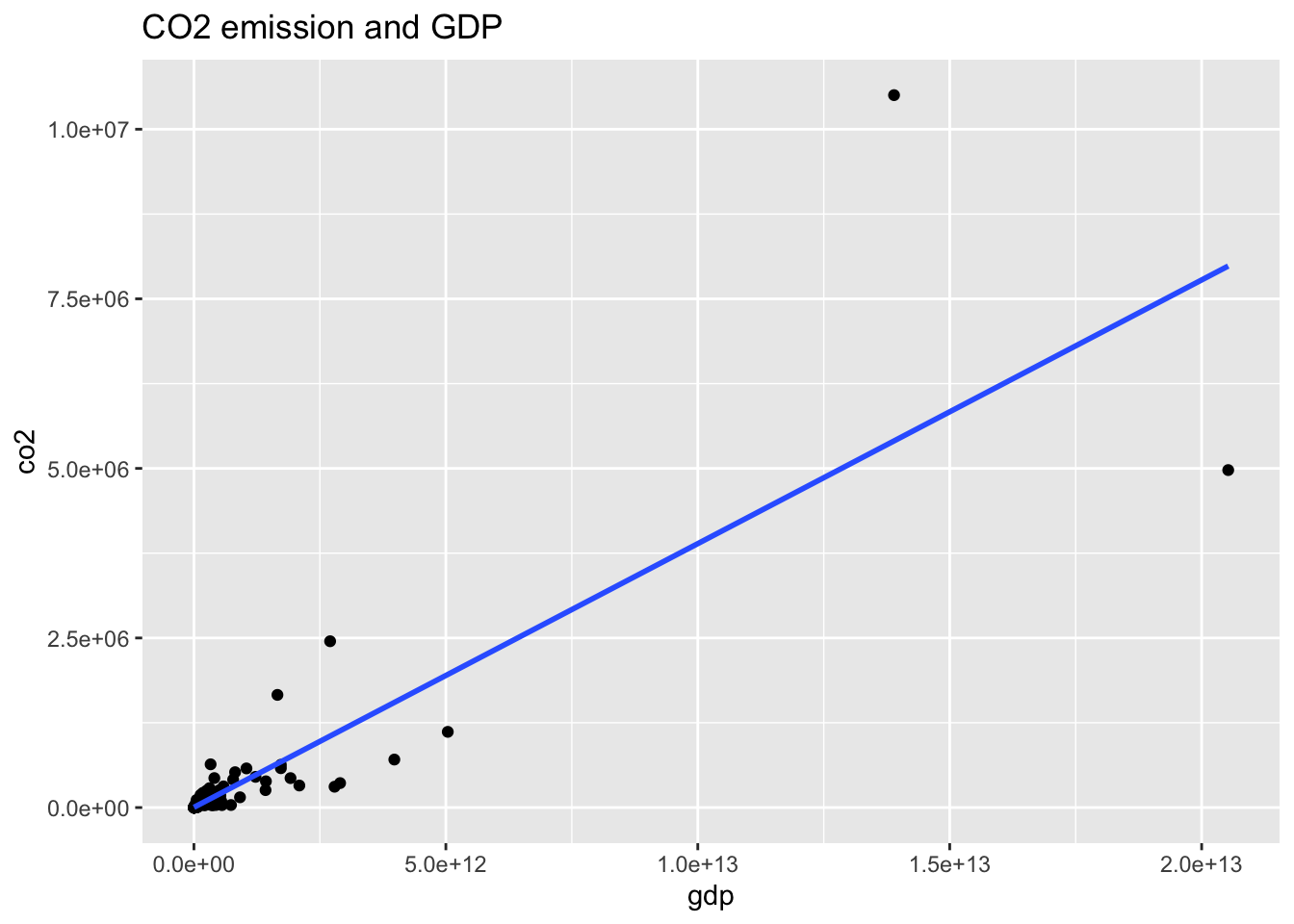

wb_co2_18 %>% ggplot(aes(gdp, co2)) + geom_point() + 
  geom_smooth(method = "lm", se = FALSE) + 
  scale_x_log10() + scale_y_log10() +
  labs(title = "CO2 emission and GDP in Log-Log scale")

## `geom_smooth()` using formula = 'y ~ x'

## Warning: Removed 4 rows containing non-finite values (`stat_smooth()`).

## Warning: Removed 4 rows containing missing values (`geom_point()`).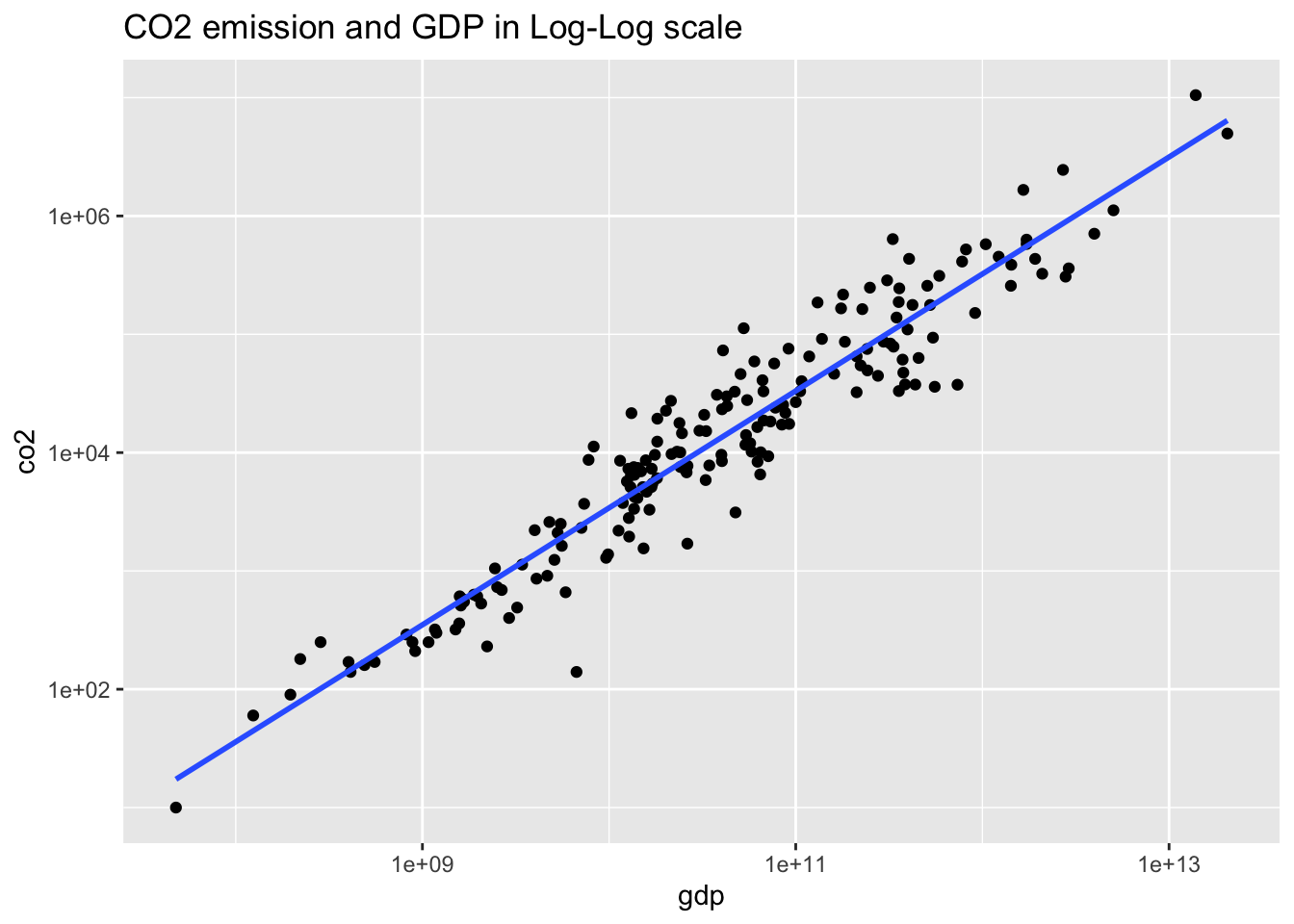

Let us take log-log plot

wb_co2_18 %>% ggplot(aes(pop, co2)) + geom_point() + 
  geom_smooth(method = "lm", se = FALSE) + 
  scale_x_log10() + scale_y_log10() +
  labs(title = "CO2 emission and Population in Log-Log scale")

## `geom_smooth()` using formula = 'y ~ x'

## Warning: Removed 1 rows containing non-finite values (`stat_smooth()`).

## Warning: Removed 1 rows containing missing values (`geom_point()`).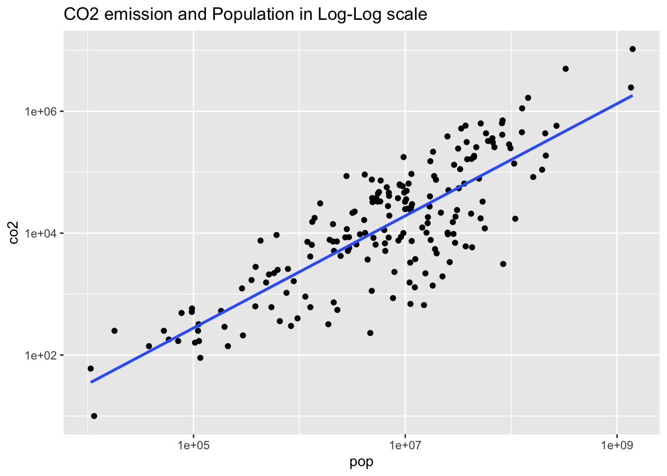

wb_co2_18 %>% ggplot(aes(cereal, co2)) + geom_point() + 
  geom_smooth(method = "lm", se = FALSE) + 
  scale_x_log10() + scale_y_log10() +
  labs(title = "CO2 emission and Land under cereal production in Log-Log scale")

## Warning: Transformation introduced infinite values in continuous x-axis
## Transformation introduced infinite values in continuous x-axis

## `geom_smooth()` using formula = 'y ~ x'

## Warning: Removed 16 rows containing non-finite values (`stat_smooth()`).

## Warning: Removed 14 rows containing missing values (`geom_point()`).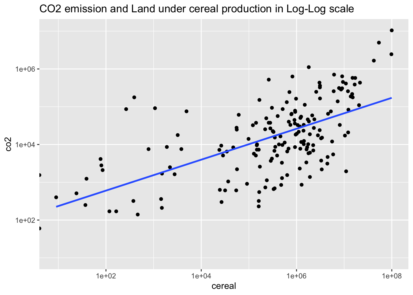

wb_co2_18m <- wb_co2_18 %>% filter(!is.na(co2), !is.na(gdp), !is.na(pop), !is.na(cereal), cereal > 0)
co2_gdp <- wb_co2_18m %>% lm(log10(co2) ~ log10(gdp), .)
co2_pop <- wb_co2_18m %>% lm(log10(co2) ~ log10(pop), .)
co2_cereal <- wb_co2_18m %>% lm(log10(co2) ~ log10(cereal), .)
co2_gdp_pop <- wb_co2_18m %>% lm(log10(co2) ~ log10(gdp) + log10(pop), .)
co2_gdp_cereal <- wb_co2_18m %>% lm(log10(co2) ~ log10(gdp) + log10(cereal), .)
co2_pop_cereal <- wb_co2_18m %>% lm(log10(co2) ~ log10(pop) + log10(cereal), .)
co2_all <- wb_co2_18m %>% lm(log10(co2) ~ log10(gdp) + log10(pop) + log10(cereal), .)

msummary(list(gdp = co2_gdp, pop = co2_pop, cereal = co2_cereal, gdp_pop = co2_gdp_pop, gdp_cereal = co2_gdp_cereal, pop_cereal = co2_pop_cereal, all = co2_all))

	gdp	pop	cereal	gdp_pop	gdp_cereal	pop_cereal	all
(Intercept)	-6.330	-2.297	1.967	-6.333	-6.136	-2.840	-6.311
	(0.271)	(0.421)	(0.240)	(0.264)	(0.279)	(0.520)	(0.292)
log10(gdp)	0.987			0.899	0.944		0.900
	(0.025)			(0.038)	(0.031)		(0.039)
log10(pop)		0.939		0.136		1.104	0.127
		(0.060)		(0.044)		(0.111)	(0.068)
log10(cereal)			0.410		0.048	-0.109	0.005
			(0.042)		(0.020)	(0.062)	(0.030)
Num.Obs.	170	170	170	170	170	170	170
R2	0.901	0.592	0.362	0.907	0.905	0.599	0.907
R2 Adj.	0.901	0.589	0.358	0.905	0.903	0.594	0.905
AIC	3683.4	3924.8	4000.7	3676.2	3679.6	3923.7	3678.1
BIC	3692.8	3934.2	4010.1	3688.7	3692.2	3936.2	3693.8
Log.Lik.	-40.453	-161.134	-199.096	-35.814	-37.559	-159.566	-35.797
RMSE	0.31	0.62	0.78	0.30	0.30	0.62	0.30

vif(co2_gdp_pop)

## log10(gdp) log10(pop) 
##   2.374532   2.374532

vif(co2_gdp_cereal)

##    log10(gdp) log10(cereal) 
##        1.5193        1.5193

vif(co2_pop_cereal)

##    log10(pop) log10(cereal) 
##      3.447368      3.447368

vif(co2_all)

##    log10(gdp)    log10(pop) log10(cereal) 
##      2.438050      5.532058      3.539584

list(gdp_pop = vif(co2_gdp_pop), gdp_cereal = vif(co2_gdp_cereal), pop_cereal = vif(co2_pop_cereal), all = vif(co2_all))

## $gdp_pop
## log10(gdp) log10(pop) 
##   2.374532   2.374532 
## 
## $gdp_cereal
##    log10(gdp) log10(cereal) 
##        1.5193        1.5193 
## 
## $pop_cereal
##    log10(pop) log10(cereal) 
##      3.447368      3.447368 
## 
## $all
##    log10(gdp)    log10(pop) log10(cereal) 
##      2.438050      5.532058      3.539584

7.3.2.1 We select regression model;

CO2 emission = c + a (GDP) + b (population)

(Omit land because of multicollinearity)

7.3.2.2 A time series data of World from 1960 to 2020

wb_co2_world <- wb_co2 %>% filter(country=="World")
wb_co2_world

## # A tibble: 61 × 16
##    country iso2c iso3c  year status lastup…¹   co2     gdp    pop  cereal region
##    <chr>   <chr> <chr> <int> <chr>  <chr>    <dbl>   <dbl>  <dbl>   <dbl> <chr> 
##  1 World   1W    WLD    1960 ""     2022-09…    NA 1.39e12 3.03e9 NA      Aggre…
##  2 World   1W    WLD    1961 ""     2022-09…    NA 1.45e12 3.07e9  5.15e8 Aggre…
##  3 World   1W    WLD    1962 ""     2022-09…    NA 1.55e12 3.12e9  5.17e8 Aggre…
##  4 World   1W    WLD    1963 ""     2022-09…    NA 1.67e12 3.19e9  5.24e8 Aggre…
##  5 World   1W    WLD    1964 ""     2022-09…    NA 1.83e12 3.26e9  5.32e8 Aggre…
##  6 World   1W    WLD    1965 ""     2022-09…    NA 1.99e12 3.32e9  5.30e8 Aggre…
##  7 World   1W    WLD    1966 ""     2022-09…    NA 2.16e12 3.39e9  5.35e8 Aggre…
##  8 World   1W    WLD    1967 ""     2022-09…    NA 2.30e12 3.46e9  5.47e8 Aggre…
##  9 World   1W    WLD    1968 ""     2022-09…    NA 2.48e12 3.53e9  5.52e8 Aggre…
## 10 World   1W    WLD    1969 ""     2022-09…    NA 2.74e12 3.61e9  5.52e8 Aggre…
## # … with 51 more rows, 5 more variables: capital <chr>, longitude <chr>,
## #   latitude <chr>, income <chr>, lending <chr>, and abbreviated variable name
## #   ¹lastupdated

wb_co2_world  %>% ggplot() + 
  geom_line(aes(x = year, y = co2)) +
  labs(title = "Co2 Emmision of the World")

## Warning: Removed 31 rows containing missing values (`geom_line()`).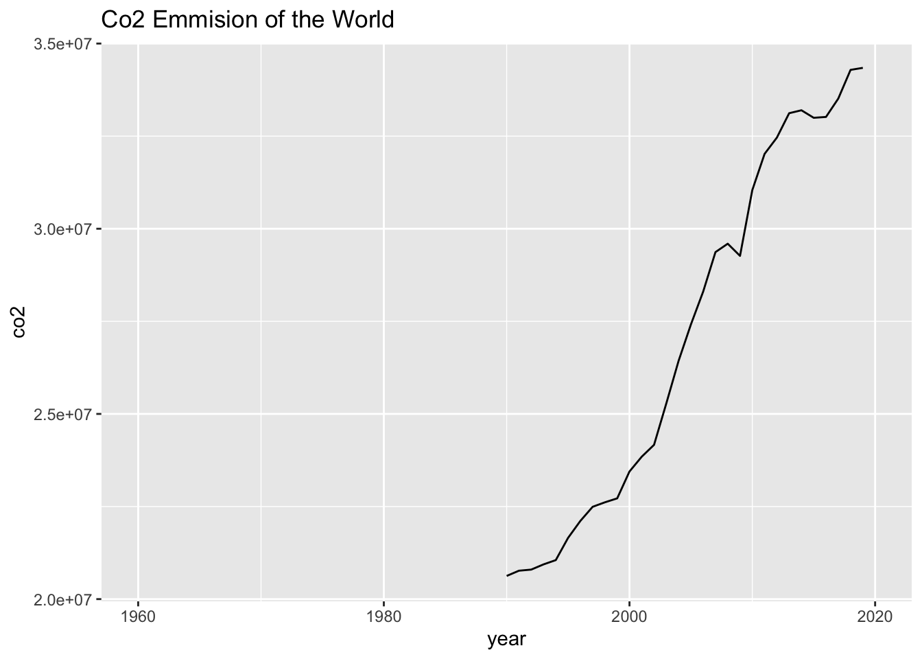

wb_co2_world %>% ggplot() + 
  geom_line(aes(x = year, y = gdp)) +
  labs(title = "GDP (current US$)")

wb_co2_world_extra <- wb_co2_world %>% 
  mutate(diff_co2 = co2 - lag(co2), diff_gdp = gdp - lag(gdp))
wb_co2_world_extra

## # A tibble: 61 × 18
##    country iso2c iso3c  year status lastup…¹   co2     gdp    pop  cereal region
##    <chr>   <chr> <chr> <int> <chr>  <chr>    <dbl>   <dbl>  <dbl>   <dbl> <chr> 
##  1 World   1W    WLD    1960 ""     2022-09…    NA 1.39e12 3.03e9 NA      Aggre…
##  2 World   1W    WLD    1961 ""     2022-09…    NA 1.45e12 3.07e9  5.15e8 Aggre…
##  3 World   1W    WLD    1962 ""     2022-09…    NA 1.55e12 3.12e9  5.17e8 Aggre…
##  4 World   1W    WLD    1963 ""     2022-09…    NA 1.67e12 3.19e9  5.24e8 Aggre…
##  5 World   1W    WLD    1964 ""     2022-09…    NA 1.83e12 3.26e9  5.32e8 Aggre…
##  6 World   1W    WLD    1965 ""     2022-09…    NA 1.99e12 3.32e9  5.30e8 Aggre…
##  7 World   1W    WLD    1966 ""     2022-09…    NA 2.16e12 3.39e9  5.35e8 Aggre…
##  8 World   1W    WLD    1967 ""     2022-09…    NA 2.30e12 3.46e9  5.47e8 Aggre…
##  9 World   1W    WLD    1968 ""     2022-09…    NA 2.48e12 3.53e9  5.52e8 Aggre…
## 10 World   1W    WLD    1969 ""     2022-09…    NA 2.74e12 3.61e9  5.52e8 Aggre…
## # … with 51 more rows, 7 more variables: capital <chr>, longitude <chr>,
## #   latitude <chr>, income <chr>, lending <chr>, diff_co2 <dbl>,
## #   diff_gdp <dbl>, and abbreviated variable name ¹lastupdated

wb_co2_world_extra %>% ggplot(aes(x = year, y = diff_co2)) + geom_line() +
  labs(title = "Changes of World CO2 emission")

## Warning: Removed 32 rows containing missing values (`geom_line()`).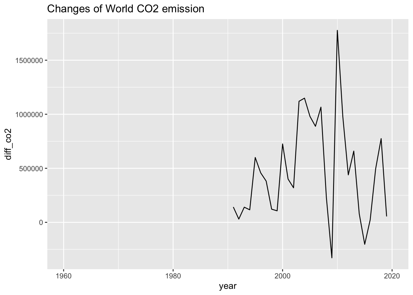

wb_co2_world_extra %>% ggplot(aes(x = year, y = diff_gdp)) + geom_line() +
  labs(title = "Changes of World GDP")

## Warning: Removed 1 row containing missing values (`geom_line()`).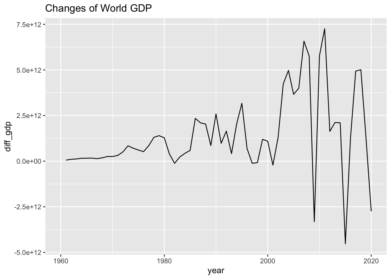

wb_co2_world_extra %>% lm(diff_co2 ~ diff_gdp, .) %>% summary()

## 
## Call:
## lm(formula = diff_co2 ~ diff_gdp, data = .)
## 
## Residuals:
##     Min      1Q  Median      3Q     Max 
## -707487 -230835  -30632  207767  839257 
## 
## Coefficients:
##              Estimate Std. Error t value Pr(>|t|)    
## (Intercept) 1.808e+05  7.780e+04   2.324   0.0279 *  
## diff_gdp    1.306e-07  2.228e-08   5.863 3.04e-06 ***
## ---
## Signif. codes:  0 '***' 0.001 '**' 0.01 '*' 0.05 '.' 0.1 ' ' 1
## 
## Residual standard error: 321600 on 27 degrees of freedom
##   ( 32 個の観測値が欠損のため削除されました )
## Multiple R-squared:  0.5601, Adjusted R-squared:  0.5438 
## F-statistic: 34.37 on 1 and 27 DF,  p-value: 3.039e-06

7.4 Regression 3: CO2 emission (Standardization)

Prof. Kaizoji provided a data in csv format in Moodle and use scale function to standardize the data, let us proceed one step by one step.
He starts with a WDI data in 2016 and use the aggregated part. There may be arguments on the set of data, let us use the same one.
He defines variance in his slides, and the codes below uses unbiased variance. The difference is minor.

 wb_co2

## # A tibble: 16,226 × 16
##    country  iso2c iso3c  year status lastu…¹   co2      gdp    pop cereal region
##    <chr>    <chr> <chr> <int> <chr>  <chr>   <dbl>    <dbl>  <dbl>  <dbl> <chr> 
##  1 Afghani… AF    AFG    2020 ""     2022-0…   NA   2.01e10 3.89e7 3.04e6 South…
##  2 Afghani… AF    AFG    2019 ""     2022-0… 6080.  1.88e10 3.80e7 2.64e6 South…
##  3 Afghani… AF    AFG    2017 ""     2022-0… 4780.  1.88e10 3.63e7 2.42e6 South…
##  4 Afghani… AF    AFG    1993 ""     2022-0… 1340  NA       1.58e7 2.63e6 South…
##  5 Afghani… AF    AFG    1983 ""     2022-0…   NA  NA       1.25e7 2.65e6 South…
##  6 Afghani… AF    AFG    2006 ""     2022-0… 1760.  6.97e 9 2.64e7 2.99e6 South…
##  7 Afghani… AF    AFG    2018 ""     2022-0… 6070.  1.81e10 3.72e7 1.91e6 South…
##  8 Afghani… AF    AFG    1981 ""     2022-0…   NA   3.48e 9 1.32e7 2.91e6 South…
##  9 Afghani… AF    AFG    2016 ""     2022-0… 5300.  1.81e10 3.54e7 2.79e6 South…
## 10 Afghani… AF    AFG    1989 ""     2022-0…   NA  NA       1.19e7 2.29e6 South…
## # … with 16,216 more rows, 5 more variables: capital <chr>, longitude <chr>,
## #   latitude <chr>, income <chr>, lending <chr>, and abbreviated variable name
## #   ¹lastupdated

co2_ag16 <- wb_co2 %>% filter(year == 2016, region=="Aggregates") %>%
  select(iso2c, co2, gdp, pop, cereal) %>% drop_na()
co2_ag16

## # A tibble: 42 × 5
##    iso2c       co2     gdp        pop    cereal
##    <chr>     <dbl>   <dbl>      <dbl>     <dbl>
##  1 ZH      578510. 8.82e11  609978946  54429019
##  2 ZI      206030. 6.91e11  412551299  57557405
##  3 1A     1838603. 2.50e12  404042892  29526231
##  4 S3       37260. 6.95e10    7269385    251540
##  5 B8      655580. 1.32e12  102994278  22398322
##  6 V2     6962022. 1.05e13 3164439749 244663698
##  7 Z4    14132393. 2.28e13 2307707227 180006919
##  8 4E    11308839. 1.36e13 2062250022 159822459
##  9 T4    11278720. 1.36e13 2036897092 158602892
## 10 XC     2255170. 1.20e13  340481755  32425857
## # … with 32 more rows

co2_al16_std <- co2_ag16 %>% mutate(st_co2 = (co2 - mean(co2))/sd(co2),
                                    st_gdp = (gdp - mean(gdp))/sd(gdp),
                                    st_pop = (pop - mean(pop))/sd(pop),
                                    st_cereal = (cereal - mean(cereal))/sd(cereal))
co2_al16_std

## # A tibble: 42 × 9
##    iso2c       co2     gdp        pop    cereal st_co2  st_gdp st_pop st_cereal
##    <chr>     <dbl>   <dbl>      <dbl>     <dbl>  <dbl>   <dbl>  <dbl>     <dbl>
##  1 ZH      578510. 8.82e11  609978946  54429019 -0.660 -0.642  -0.487   -0.546 
##  2 ZI      206030. 6.91e11  412551299  57557405 -0.708 -0.654  -0.593   -0.528 
##  3 1A     1838603. 2.50e12  404042892  29526231 -0.498 -0.541  -0.598   -0.692 
##  4 S3       37260. 6.95e10    7269385    251540 -0.730 -0.693  -0.812   -0.863 
##  5 B8      655580. 1.32e12  102994278  22398322 -0.651 -0.615  -0.760   -0.733 
##  6 V2     6962022. 1.05e13 3164439749 244663698  0.162 -0.0451  0.893    0.567 
##  7 Z4    14132393. 2.28e13 2307707227 180006919  1.09   0.723   0.430    0.189 
##  8 4E    11308839. 1.36e13 2062250022 159822459  0.723  0.152   0.298    0.0706
##  9 T4    11278720. 1.36e13 2036897092 158602892  0.719  0.151   0.284    0.0635
## 10 XC     2255170. 1.20e13  340481755  32425857 -0.444  0.0495 -0.632   -0.675 
## # … with 32 more rows

co2_al16_scaled <- co2_ag16 %>% mutate(st_co2 = scale(co2),
                                    st_gdp = scale(gdp),
                                    st_pop = scale(pop),
                                    st_cereal = scale(cereal))
co2_al16_scaled

## # A tibble: 42 × 9
##    iso2c       co2     gdp        pop    cereal st_co2…¹ st_gd…² st_po…³ st_ce…⁴
##    <chr>     <dbl>   <dbl>      <dbl>     <dbl>    <dbl>   <dbl>   <dbl>   <dbl>
##  1 ZH      578510. 8.82e11  609978946  54429019   -0.660 -0.642   -0.487 -0.546 
##  2 ZI      206030. 6.91e11  412551299  57557405   -0.708 -0.654   -0.593 -0.528 
##  3 1A     1838603. 2.50e12  404042892  29526231   -0.498 -0.541   -0.598 -0.692 
##  4 S3       37260. 6.95e10    7269385    251540   -0.730 -0.693   -0.812 -0.863 
##  5 B8      655580. 1.32e12  102994278  22398322   -0.651 -0.615   -0.760 -0.733 
##  6 V2     6962022. 1.05e13 3164439749 244663698    0.162 -0.0451   0.893  0.567 
##  7 Z4    14132393. 2.28e13 2307707227 180006919    1.09   0.723    0.430  0.189 
##  8 4E    11308839. 1.36e13 2062250022 159822459    0.723  0.152    0.298  0.0706
##  9 T4    11278720. 1.36e13 2036897092 158602892    0.719  0.151    0.284  0.0635
## 10 XC     2255170. 1.20e13  340481755  32425857   -0.444  0.0495  -0.632 -0.675 
## # … with 32 more rows, and abbreviated variable names ¹st_co2[,1], ²st_gdp[,1],
## #   ³st_pop[,1], ⁴st_cereal[,1]

co2_ag16 %>% select(-1) %>% scale() %>% as_tibble()

## # A tibble: 42 × 4
##       co2     gdp    pop  cereal
##     <dbl>   <dbl>  <dbl>   <dbl>
##  1 -0.660 -0.642  -0.487 -0.546 
##  2 -0.708 -0.654  -0.593 -0.528 
##  3 -0.498 -0.541  -0.598 -0.692 
##  4 -0.730 -0.693  -0.812 -0.863 
##  5 -0.651 -0.615  -0.760 -0.733 
##  6  0.162 -0.0451  0.893  0.567 
##  7  1.09   0.723   0.430  0.189 
##  8  0.723  0.152   0.298  0.0706
##  9  0.719  0.151   0.284  0.0635
## 10 -0.444  0.0495 -0.632 -0.675 
## # … with 32 more rows

co2_ag16_rv <- read_csv("data/AGCO2rv.csv")

## Rows: 44 Columns: 4
## ── Column specification ──────────────────────────────────────────────────────────────────────────────────────────────────────
## Delimiter: ","
## dbl (4): EN.ATM.CO2E.KT, NY.GDP.MKTP.CD, SP.POP.TOTL, AG.LND.CREL.HA
## 
## ℹ Use `spec()` to retrieve the full column specification for this data.
## ℹ Specify the column types or set `show_col_types = FALSE` to quiet this message.

co2_ag16_rv

## # A tibble: 44 × 4
##    EN.ATM.CO2E.KT NY.GDP.MKTP.CD SP.POP.TOTL AG.LND.CREL.HA
##             <dbl>          <dbl>       <dbl>          <dbl>
##  1       1846601.        2.40e12   404042892       29143572
##  2      32940650.        7.63e13  7433569330      733367261
##  3      11254611.        1.36e13  2062232304      163412028
##  4       2837305.        2.97e12   412538477      104861504
##  5       2479230         2.93e12  1771187426      132269014
##  6        656330         1.32e12   102994278       22398321
##  7       2904100         1.39e13   445487730       54059756
##  8        733332.        1.41e12   849739853       95574606
##  9      11961830         4.84e13  1341701902      165097397
## 10        228009.        4.45e11    39198032        1809678
## # … with 34 more rows

colnames(co2_ag16_rv) <- c("st_co2", "st_gdp", "st_pop", "st_cereal")
co2_ag16_rv

## # A tibble: 44 × 4
##       st_co2  st_gdp     st_pop st_cereal
##        <dbl>   <dbl>      <dbl>     <dbl>
##  1  1846601. 2.40e12  404042892  29143572
##  2 32940650. 7.63e13 7433569330 733367261
##  3 11254611. 1.36e13 2062232304 163412028
##  4  2837305. 2.97e12  412538477 104861504
##  5  2479230  2.93e12 1771187426 132269014
##  6   656330  1.32e12  102994278  22398321
##  7  2904100  1.39e13  445487730  54059756
##  8   733332. 1.41e12  849739853  95574606
##  9 11961830  4.84e13 1341701902 165097397
## 10   228009. 4.45e11   39198032   1809678
## # … with 34 more rows

7.4.1 Regression

co2_al16_scaled  %>% ggplot(aes(st_gdp, st_co2)) + geom_point() + 
  geom_smooth(method = "lm", se = FALSE) + 
  labs(title = "CO2 emission and GDP: Standardized")

## `geom_smooth()` using formula = 'y ~ x'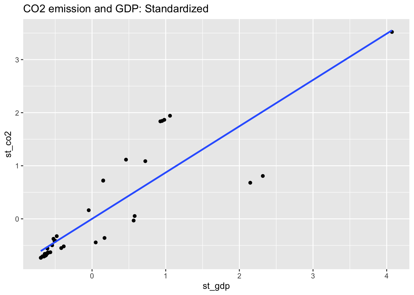

co2_al16_scaled  %>% ggplot(aes(st_pop, st_co2)) + geom_point() + 
  geom_smooth(method = "lm", se = FALSE) + 
  labs(title = "CO2 emission and Population: Standardized")

## `geom_smooth()` using formula = 'y ~ x'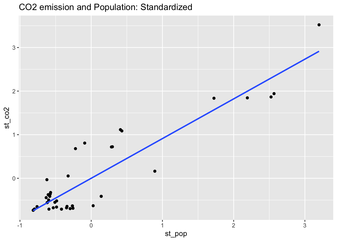

co2_al16_scaled  %>% ggplot(aes(st_cereal, st_co2)) + geom_point() + 
  geom_smooth(method = "lm", se = FALSE) + 
  labs(title = "CO2 emission and Land under cereal production: Standardized")

## `geom_smooth()` using formula = 'y ~ x'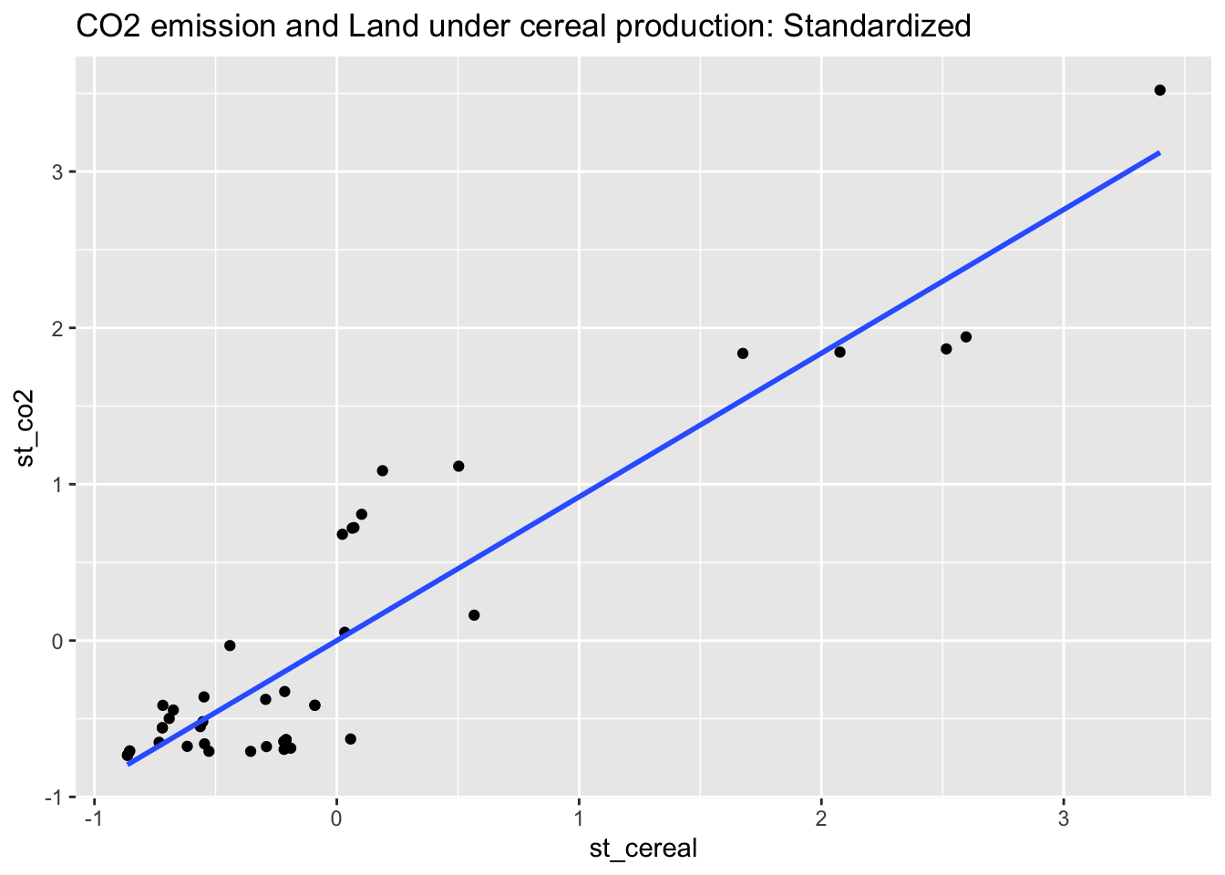

st_co2_gdp <- co2_al16_scaled  %>% lm(st_co2 ~ st_gdp, .)
st_co2_pop <- co2_al16_scaled  %>% lm(st_co2 ~ st_pop, .)
st_co2_cereal <- co2_al16_scaled  %>% lm(st_co2 ~ st_cereal, .)
st_co2_gdp_pop <- co2_al16_scaled %>% lm(st_co2 ~ st_gdp + st_pop, .)
st_co2_gdp_cereal <- co2_al16_scaled  %>% lm(st_co2 ~ st_gdp + st_cereal, .)
st_co2_pop_cereal <- co2_al16_scaled  %>% lm(st_co2 ~ st_pop + st_cereal, .)
st_co2_all <- co2_al16_scaled  %>% lm(st_co2 ~ st_gdp + st_pop + st_cereal, .)

msummary(list(st_gdp = st_co2_gdp, st_pop = st_co2_pop, st_cereal = st_co2_cereal, st_gdp_pop = st_co2_gdp_pop, st_gdp_cereal = st_co2_gdp_cereal, st_pop_cereal = st_co2_pop_cereal, st_all = st_co2_all))

	st_gdp	st_pop	st_cereal	st_gdp_pop	st_gdp_cereal	st_pop_cereal	st_all
(Intercept)	8e-17	2e-17	7e-17	5e-17	8e-17	6e-17	4e-17
	(0.076)	(0.064)	(0.062)	(0.038)	(0.042)	(0.062)	(0.038)
st_gdp	0.872			0.464	0.427		0.491
	(0.077)			(0.053)	(0.063)		(0.060)
st_pop		0.911		0.590		0.142	0.829
		(0.065)		(0.053)		(0.397)	(0.257)
st_cereal			0.919		0.605	0.779	-0.261
			(0.062)		(0.063)	(0.397)	(0.274)
Num.Obs.	42	42	42	42	42	42	42
R2	0.761	0.830	0.845	0.942	0.928	0.845	0.944
R2 Adj.	0.755	0.826	0.841	0.939	0.924	0.837	0.939
AIC	64.1	49.8	46.0	6.4	15.6	47.9	7.4
BIC	69.3	55.0	51.2	13.4	22.6	54.8	16.1
Log.Lik.	-29.067	-21.908	-19.997	0.784	-3.806	-19.928	1.278
RMSE	0.48	0.41	0.39	0.24	0.26	0.39	0.23

vif(st_co2_gdp_pop)

##   st_gdp   st_pop 
## 1.916177 1.916177

vif(st_co2_gdp_cereal)

##    st_gdp st_cereal 
##  2.182838  2.182838

vif(st_co2_pop_cereal)

##    st_pop st_cereal 
##  39.64498  39.64498

vif(st_co2_all)

##    st_gdp    st_pop st_cereal 
##  2.446917 44.441219 50.625778

7.4.2 Not Standardized

co2_al16 <- wb_co2 %>% filter(region != "Aggregates", year == 2016)
co2_al16

## # A tibble: 216 × 16
##    country       iso2c iso3c  year status lastu…¹     co2     gdp    pop  cereal
##    <chr>         <chr> <chr> <int> <chr>  <chr>     <dbl>   <dbl>  <dbl>   <dbl>
##  1 Afghanistan   AF    AFG    2016 ""     2022-0…   5300. 1.81e10 3.54e7  2.79e6
##  2 Albania       AL    ALB    2016 ""     2022-0…   4480. 1.19e10 2.88e6  1.48e5
##  3 Algeria       DZ    DZA    2016 ""     2022-0… 154910. 1.60e11 4.06e7  3.38e6
##  4 American Sam… AS    ASM    2016 ""     2022-0…     NA  6.71e 8 5.57e4 NA     
##  5 Andorra       AD    AND    2016 ""     2022-0…    470. 2.90e 9 7.73e4 NA     
##  6 Angola        AO    AGO    2016 ""     2022-0…  29760. 4.98e10 2.88e7  2.73e6
##  7 Antigua and … AG    ATG    2016 ""     2022-0…    500  1.44e 9 9.45e4  3.5 e1
##  8 Argentina     AR    ARG    2016 ""     2022-0… 183160. 5.58e11 4.36e7  1.18e7
##  9 Armenia       AM    ARM    2016 ""     2022-0…   5070. 1.05e10 2.94e6  1.95e5
## 10 Aruba         AW    ABW    2016 ""     2022-0…     NA  2.98e 9 1.05e5 NA     
## # … with 206 more rows, 6 more variables: region <chr>, capital <chr>,
## #   longitude <chr>, latitude <chr>, income <chr>, lending <chr>, and
## #   abbreviated variable name ¹lastupdated

7.4.3 Regression

co2_al16 %>% ggplot(aes(gdp, co2)) + geom_point() + 
  geom_smooth(method = "lm", se = FALSE) + 
  labs(title = "CO2 emission and GDP")

## `geom_smooth()` using formula = 'y ~ x'

## Warning: Removed 30 rows containing non-finite values (`stat_smooth()`).

## Warning: Removed 30 rows containing missing values (`geom_point()`).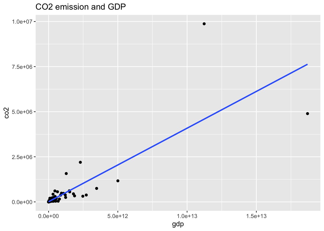

co2_al16 %>% ggplot(aes(pop, co2)) + geom_point() + 
  geom_smooth(method = "lm", se = FALSE) + 
  labs(title = "CO2 emission and Population")

## `geom_smooth()` using formula = 'y ~ x'

## Warning: Removed 27 rows containing non-finite values (`stat_smooth()`).

## Warning: Removed 27 rows containing missing values (`geom_point()`).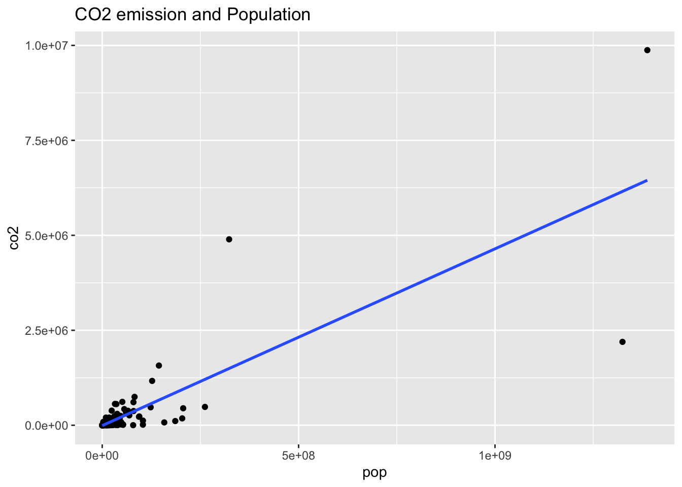

co2_al16 %>% ggplot(aes(cereal, co2)) + geom_point() + 
  geom_smooth(method = "lm", se = FALSE) + 
  labs(title = "CO2 emission and Land under cereal production")

## `geom_smooth()` using formula = 'y ~ x'

## Warning: Removed 41 rows containing non-finite values (`stat_smooth()`).

## Warning: Removed 41 rows containing missing values (`geom_point()`).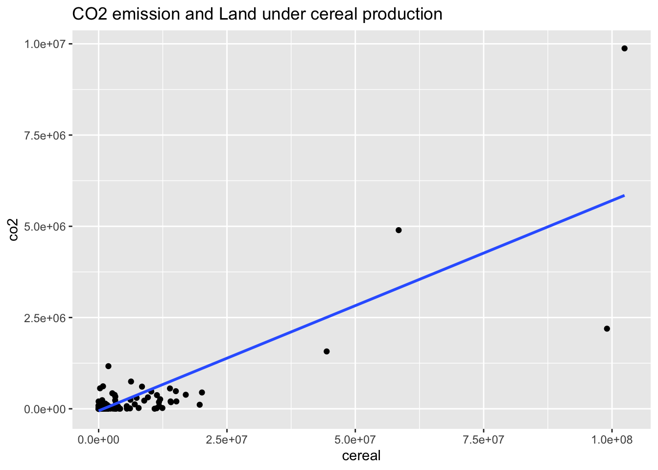

orig_co2_gdp <- wb_co2_18 %>% lm(co2 ~ gdp, .)
orig_co2_pop <- wb_co2_18 %>% lm(co2 ~ pop, .)
orig_co2_cereal <- wb_co2_18 %>% lm(co2 ~ cereal, .)
orig_co2_gdp_pop <- wb_co2_18 %>% lm(co2 ~ gdp + pop, .)
orig_co2_gdp_cereal <- wb_co2_18 %>% lm(co2 ~ gdp + cereal, .)
orig_co2_pop_cereal <- wb_co2_18 %>% lm(co2 ~ pop + cereal, .)
orig_co2_all <- wb_co2_18 %>% lm(co2 ~ gdp + pop + cereal, .)

msummary(list(orog_gdp = orig_co2_gdp, orig_pop = orig_co2_pop, orig_cereal = orig_co2_cereal, orig_gdp_pop = orig_co2_gdp_pop, orig_gdp_cereal = orig_co2_gdp_cereal, orig_pop_cereal = orig_co2_pop_cereal, orig_all = orig_co2_all))

	orog_gdp	orig_pop	orig_cereal	orig_gdp_pop	orig_gdp_cereal	orig_pop_cereal	orig_all
(Intercept)	3515.953	-15951.506	-63228.012	-55340.997	-73957.970	-52752.510	-55825.130
	(35988.776)	(38195.903)	(40611.145)	(24242.415)	(30130.231)	(40260.650)	(26764.555)
gdp	0.0000004			0.0000003	0.0000002		0.0000003
	(2e-08)			(1e-08)	(2e-08)		(2e-08)
pop		0.005		0.003		0.002	0.003
		(0.0003)		(0.0002)		(0.0007)	(0.0005)
cereal			0.062		0.036	0.039	-0.005
			(0.003)		(0.003)	(0.009)	(0.007)
Num.Obs.	186	189	176	186	172	175	172
R2	0.708	0.666	0.684	0.871	0.835	0.697	0.872
R2 Adj.	0.706	0.664	0.682	0.870	0.833	0.694	0.870
AIC	5396.1	5505.5	5129.4	5245.3	4906.9	5095.6	4865.5
BIC	5405.8	5515.2	5138.9	5258.2	4919.5	5108.2	4881.2
Log.Lik.	-2695.047	-2749.741	-2561.711	-2618.668	-2449.437	-2543.785	-2427.731
RMSE	474757.79	503810.82	506985.87	314872.13	370265.90	497313.02	326367.04

vif(orig_co2_gdp_pop)

##      gdp      pop 
## 1.498289 1.498289

vif(orig_co2_gdp_cereal)

##      gdp   cereal 
## 1.795285 1.795285

vif(orig_co2_pop_cereal)

##      pop   cereal 
## 8.098126 8.098126

vif(orig_co2_all)

##       gdp       pop    cereal 
##  1.859018  8.401085 10.101136

7.4.3.1 Standadized (Again)

msummary(list(st_gdp = st_co2_gdp, st_pop = st_co2_pop, st_cereal = st_co2_cereal, st_gdp_pop = st_co2_gdp_pop, st_gdp_cereal = st_co2_gdp_cereal, st_pop_cereal = st_co2_pop_cereal, st_all = st_co2_all))

	st_gdp	st_pop	st_cereal	st_gdp_pop	st_gdp_cereal	st_pop_cereal	st_all
(Intercept)	8e-17	2e-17	7e-17	5e-17	8e-17	6e-17	4e-17
	(0.076)	(0.064)	(0.062)	(0.038)	(0.042)	(0.062)	(0.038)
st_gdp	0.872			0.464	0.427		0.491
	(0.077)			(0.053)	(0.063)		(0.060)
st_pop		0.911		0.590		0.142	0.829
		(0.065)		(0.053)		(0.397)	(0.257)
st_cereal			0.919		0.605	0.779	-0.261
			(0.062)		(0.063)	(0.397)	(0.274)
Num.Obs.	42	42	42	42	42	42	42
R2	0.761	0.830	0.845	0.942	0.928	0.845	0.944
R2 Adj.	0.755	0.826	0.841	0.939	0.924	0.837	0.939
AIC	64.1	49.8	46.0	6.4	15.6	47.9	7.4
BIC	69.3	55.0	51.2	13.4	22.6	54.8	16.1
Log.Lik.	-29.067	-21.908	-19.997	0.784	-3.806	-19.928	1.278
RMSE	0.48	0.41	0.39	0.24	0.26	0.39	0.23

vif(st_co2_gdp_pop)

##   st_gdp   st_pop 
## 1.916177 1.916177

vif(st_co2_gdp_cereal)

##    st_gdp st_cereal 
##  2.182838  2.182838

vif(st_co2_pop_cereal)

##    st_pop st_cereal 
##  39.64498  39.64498

vif(st_co2_all)

##    st_gdp    st_pop st_cereal 
##  2.446917 44.441219 50.625778

7.4.4 We select regression model;

CO2 emission = c + a (GDP) + b (population)
(Omit land because of multicollinearity)

7.5 Regression of Categorical Variables and ANOVA

If you start from here, you need to load the following packages.

library(tidyverse) #tidyverse Package, a collection of packages for data science
library(WDI) #WDI Package for World Development Indicators
library(car) #VIF function
library(modelsummary) #Table of the regression results

wb_co2

## # A tibble: 16,226 × 16
##    country  iso2c iso3c  year status lastu…¹   co2      gdp    pop cereal region
##    <chr>    <chr> <chr> <int> <chr>  <chr>   <dbl>    <dbl>  <dbl>  <dbl> <chr> 
##  1 Afghani… AF    AFG    2020 ""     2022-0…   NA   2.01e10 3.89e7 3.04e6 South…
##  2 Afghani… AF    AFG    2019 ""     2022-0… 6080.  1.88e10 3.80e7 2.64e6 South…
##  3 Afghani… AF    AFG    2017 ""     2022-0… 4780.  1.88e10 3.63e7 2.42e6 South…
##  4 Afghani… AF    AFG    1993 ""     2022-0… 1340  NA       1.58e7 2.63e6 South…
##  5 Afghani… AF    AFG    1983 ""     2022-0…   NA  NA       1.25e7 2.65e6 South…
##  6 Afghani… AF    AFG    2006 ""     2022-0… 1760.  6.97e 9 2.64e7 2.99e6 South…
##  7 Afghani… AF    AFG    2018 ""     2022-0… 6070.  1.81e10 3.72e7 1.91e6 South…
##  8 Afghani… AF    AFG    1981 ""     2022-0…   NA   3.48e 9 1.32e7 2.91e6 South…
##  9 Afghani… AF    AFG    2016 ""     2022-0… 5300.  1.81e10 3.54e7 2.79e6 South…
## 10 Afghani… AF    AFG    1989 ""     2022-0…   NA  NA       1.19e7 2.29e6 South…
## # … with 16,216 more rows, 5 more variables: capital <chr>, longitude <chr>,
## #   latitude <chr>, income <chr>, lending <chr>, and abbreviated variable name
## #   ¹lastupdated

wb_co2_4anova <- wb_co2 %>% filter(year == 2016, region != "Aggregates") %>%
  select(iso2c, co2, gdp, income) %>% drop_na() %>%
  mutate(log_co2 = log10(co2), log_gdp = log10(gdp))
wb_co2_4anova

## # A tibble: 186 × 6
##    iso2c     co2     gdp income              log_co2 log_gdp
##    <chr>   <dbl>   <dbl> <chr>                 <dbl>   <dbl>
##  1 AF      5300. 1.81e10 Low income             3.72   10.3 
##  2 AL      4480. 1.19e10 Upper middle income    3.65   10.1 
##  3 DZ    154910. 1.60e11 Lower middle income    5.19   11.2 
##  4 AD       470. 2.90e 9 High income            2.67    9.46
##  5 AO     29760. 4.98e10 Lower middle income    4.47   10.7 
##  6 AG       500  1.44e 9 High income            2.70    9.16
##  7 AR    183160. 5.58e11 Upper middle income    5.26   11.7 
##  8 AM      5070. 1.05e10 Upper middle income    3.71   10.0 
##  9 AU    384990. 1.21e12 High income            5.59   12.1 
## 10 AT     63680. 3.96e11 High income            4.80   11.6 
## # … with 176 more rows

CO2 <- as_tibble(read.csv("CO2CAPITA.csv"))
CO2
str(CO2)
head(CO2)
tail(CO2)

wb_co2_4anova %>% group_by(income) %>% 
  summarize(n = n_distinct(iso2c), co2_mean = mean(co2), gdp_mean = mean(gdp), log_co2_mean = mean(log_co2), log_gdp_mean = mean(log_gdp))

## # A tibble: 4 × 6
##   income                  n co2_mean      gdp_mean log_co2_mean log_gdp_mean
##   <chr>               <int>    <dbl>         <dbl>        <dbl>        <dbl>
## 1 High income            56  217188. 857319296294.         4.46        11.1 
## 2 Low income             25    5053.  17841983559.         3.39         9.99
## 3 Lower middle income    53   96503. 129620974752.         3.98        10.3 
## 4 Upper middle income    52  286264. 375800809797.         4.10        10.4

7.5.1 Regression

y <- CO2$EN.ATM.CO2E.PC #CO2 Emission per capita
x <- CO2$NY.GDP.PCAP.PP.CD/10000 #GDP per capita, PPP
summary(x)
summary(y)

wb_co2_4anova %>% ggplot(aes(log_gdp, log_co2)) +
  geom_point() +
  geom_smooth(method = "lm", se = FALSE) +
  labs(title = "CO2 emission per capita and GDP per capita in log-log scale", 
       x = "GDP per capita", y = "CO2 emission per capita")

## `geom_smooth()` using formula = 'y ~ x'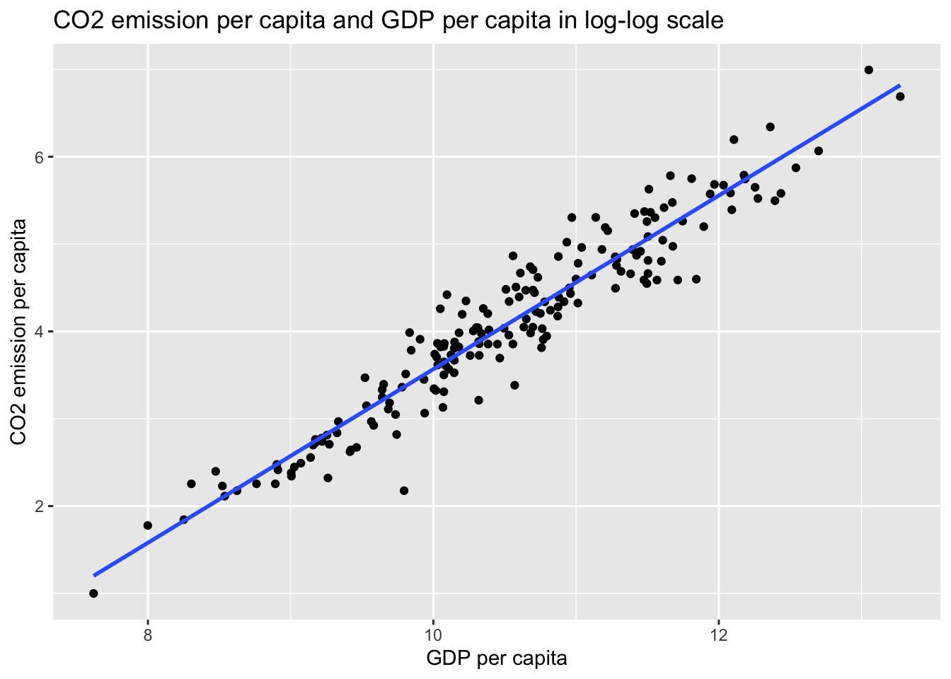

CO2 %>% ggplot(aes(x, y)) +
  geom_point() +
  geom_smooth(method = "lm", se = FALSE) +
  labs(title = "CO2 emission per capita and GDP per capita", 
       x = "GDP per capita", y = "CO2 emission per capita")

model_1 <-lm(y ~ x, data=CO2)
summary(model_1)
msummary(model_1, statistic = 'p.value')

wb_co2_4anova %>% ggplot(aes(x = log_co2, fill =  income)) + 
  geom_histogram( )

## `stat_bin()` using `bins = 30`. Pick better value with `binwidth`.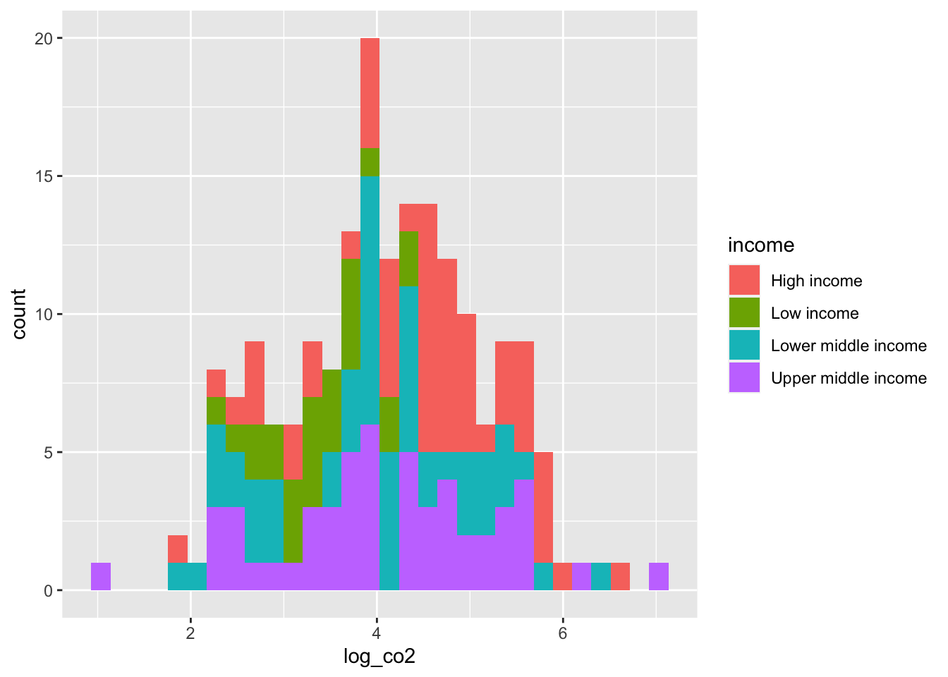

wb_co2_4anova %>% ggplot(aes(x = log_co2, y = income, fill =  income)) + 
  geom_boxplot()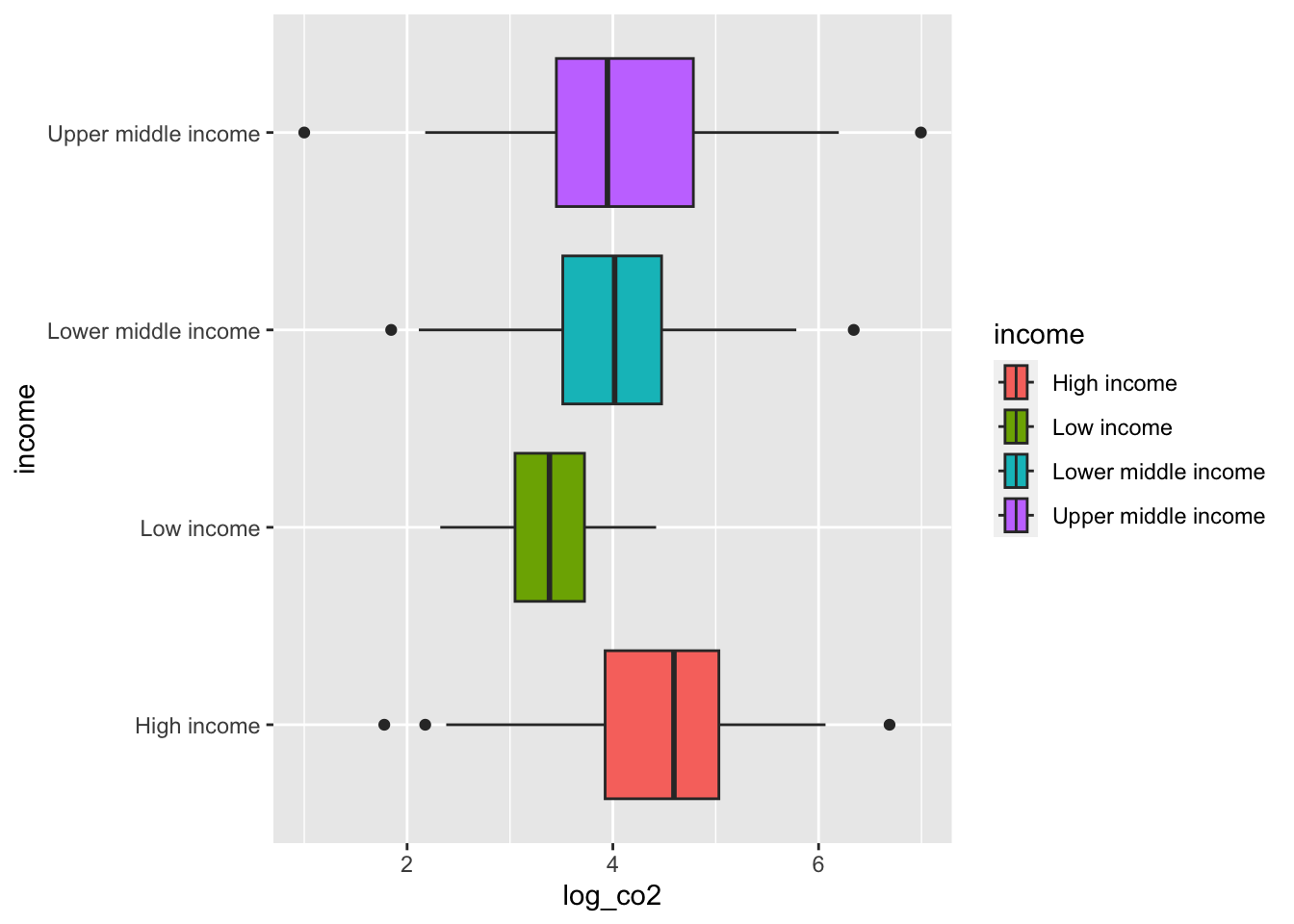

wb_co2_anova <- wb_co2_4anova %>% mutate(hi = as.numeric(income == "High income"))

wb_co2_model <- wb_co2_anova %>% lm(co2 ~ gdp + hi, .)
wb_co2_model %>% summary()

## 
## Call:
## lm(formula = co2 ~ gdp + hi, data = .)
## 
## Residuals:
##      Min       1Q   Median       3Q      Max 
## -2775444   -69456   -66758    54673  5112814 
## 
## Coefficients:
##               Estimate Std. Error t value Pr(>|t|)    
## (Intercept)  6.850e+04  4.110e+04   1.667  0.09727 .  
## gdp          4.178e-07  2.066e-08  20.221  < 2e-16 ***
## hi          -2.095e+05  7.570e+04  -2.768  0.00623 ** 
## ---
## Signif. codes:  0 '***' 0.001 '**' 0.01 '*' 0.05 '.' 0.1 ' ' 1
## 
## Residual standard error: 466100 on 183 degrees of freedom
## Multiple R-squared:  0.6912, Adjusted R-squared:  0.6878 
## F-statistic: 204.8 on 2 and 183 DF,  p-value: < 2.2e-16

wb_co2_log_model <- wb_co2_anova %>% lm(log_co2 ~ log_gdp + hi, .)
wb_co2_log_model %>% summary()

## 
## Call:
## lm(formula = log_co2 ~ log_gdp + hi, data = .)
## 
## Residuals:
##      Min       1Q   Median       3Q      Max 
## -0.97183 -0.19548 -0.02953  0.16620  0.69532 
## 
## Coefficients:
##             Estimate Std. Error t value Pr(>|t|)    
## (Intercept) -6.72924    0.23113 -29.114  < 2e-16 ***
## log_gdp      1.03559    0.02235  46.337  < 2e-16 ***
## hi          -0.26638    0.05022  -5.304 3.24e-07 ***
## ---
## Signif. codes:  0 '***' 0.001 '**' 0.01 '*' 0.05 '.' 0.1 ' ' 1
## 
## Residual standard error: 0.2943 on 183 degrees of freedom
## Multiple R-squared:  0.9258, Adjusted R-squared:  0.925 
## F-statistic:  1142 on 2 and 183 DF,  p-value: < 2.2e-16

income_model <- wb_co2_anova %>% lm(co2 ~ factor(income), .) 
income_model %>% summary()

## 
## Call:
## lm(formula = co2 ~ factor(income), data = .)
## 
## Residuals:
##     Min      1Q  Median      3Q     Max 
## -286254 -215768  -96018   -3903 9588396 
## 
## Coefficients:
##                                   Estimate Std. Error t value Pr(>|t|)  
## (Intercept)                         217188     111597   1.946   0.0532 .
## factor(income)Low income           -212135     200875  -1.056   0.2923  
## factor(income)Lower middle income  -120685     160040  -0.754   0.4518  
## factor(income)Upper middle income    69076     160829   0.429   0.6681  
## ---
## Signif. codes:  0 '***' 0.001 '**' 0.01 '*' 0.05 '.' 0.1 ' ' 1
## 
## Residual standard error: 835100 on 182 degrees of freedom
## Multiple R-squared:  0.01392,    Adjusted R-squared:  -0.002335 
## F-statistic: 0.8563 on 3 and 182 DF,  p-value: 0.4649

msummary(list(co2_model = wb_co2_model, co2_log_model = wb_co2_log_model, co2_income_model = income_model), statistic = 'p.value')

	co2_model	co2_log_model	co2_income_model
(Intercept)	68502.943	-6.729	217187.858
	(0.097)	(<0.001)	(0.053)
gdp	0.0000004
	(<0.001)
hi	-209509.183	-0.266
	(0.006)	(<0.001)
log_gdp		1.036
		(<0.001)
factor(income)Low income			-212135.058
			(0.292)
factor(income)Lower middle income			-120685.215
			(0.452)
factor(income)Upper middle income			69075.992
			(0.668)
Num.Obs.	186	186	186
R2	0.691	0.926	0.014
R2 Adj.	0.688	0.925	-0.002
AIC	5388.2	77.7	5606.1
BIC	5401.1	90.7	5622.3
Log.Lik.	-2690.100	-34.874	-2798.072
RMSE	462298.61	0.29	826089.87

7.5.1.1 t-test

high <- wb_co2_4anova %>% filter(income == "High income") %>% pull(co2)
low <- wb_co2_4anova %>% filter(income == "Low income") %>% pull(co2)
t.test(high, low)

## 
##  Welch Two Sample t-test
## 
## data:  high and low
## t = 2.3527, df = 55.024, p-value = 0.02224
## alternative hypothesis: true difference in means is not equal to 0
## 95 percent confidence interval:
##   31435.4 392834.7
## sample estimates:
## mean of x mean of y 
##  217187.9    5052.8

7.5.2 Regression analysis with categorical variables

model_3=lm(EN.ATM.CO2E.PC ~ factor(income), data = CO2)

summary(model_3) # summary

msummary(model_3, statistic = ‘p.value’)

7.5.3 ANOVA (Analysis of Variance)

wb_co2_4anova %>% aov(co2 ~ factor(income), .) %>% summary()

##                 Df    Sum Sq   Mean Sq F value Pr(>F)
## factor(income)   3 1.792e+12 5.972e+11   0.856  0.465
## Residuals      182 1.269e+14 6.974e+11

7.6 Week 7 Assignment

Week 7: Assignment on regression analysis and PPDAC cycle
Work on the following problem.
Problem: Find one problem from the SGDs goal.
Example: WDI environment
https://datatopics.worldbank.org/world-development-indicators/themes/environment.html
Plan: Analyze the data to find out why the problem is occurring.
Data: Collect data from WDI and other sources (OECD, UN, IMF, etc.).
Analysis: Analyze the data. Use what you have learned about regression analysis and descriptive statistics in the previous lectures.
Conclusion: Briefly describe what you learn from the data analysis.
Submission: Your rmd file (Rmarkdown) on Moodle box.

*Deadline : Feb. 8.

Chapter 7 Topics in Exploratory Data Analysis I

Summary

Dot Place Holder in lm.

7.1 Part I: Regression 1:

7.1.1 Why does GDP vary from country to country?

7.1.2 Regression

7.1.3 Checking for multicollinearity

7.1.4 vif: Determination of multi-collinearity

7.1.4.1 VIF (Variance Inflation Factor)

7.1.4.2 Conclusion

7.2 A time series data of World from 1960 to 2020

7.2.1 Excercise:

7.3 Regression 2 : CO2 Emission

7.3.1 Project

7.3.1.1 Regression Analysis

7.3.1.2 WDI Indicator cordes

7.3.2 Regression

7.3.2.1 We select regression model;

7.3.2.2 A time series data of World from 1960 to 2020

7.4 Regression 3: CO2 emission (Standardization)

7.4.1 Regression

7.4.2 Not Standardized

7.4.3 Regression

7.4.3.1 Standadized (Again)

7.4.4 We select regression model;

7.5 Regression of Categorical Variables and ANOVA

7.5.1 Regression

7.5.1.1 t-test

7.5.2 Regression analysis with categorical variables

7.5.3 ANOVA (Analysis of Variance)

7.6 Week 7 Assignment

Chapter 7 Topics in Exploratory Data Analysis I　

Dot Place Holder in `lm`.