Chapter 6 Exploratory Data Analysis (EDA) 5

Course Contents

2021-12-08: Introduction: About the course
- An introduction to open and public data, and data science
2021-12-15: Exploratory Data Analysis (EDA) 1 [lead by hs]
- R Basics with RStudio and/or RStudio.cloud; R Script, swirl
2021-12-22: Exploratory Data Analysis (EDA) 2 [lead by hs]
- R Markdown; Introduction to tidyverse; RStudio Primers
2022-01-12: Exploratory Data Analysis (EDA) 3 [lead by hs]
- Introduction to tidyverse; Public Data, WDI, etc
2022-01-19: Exploratory Data Analysis (EDA) 4 [lead by hs]
- Introduction to tidyverse; WDI, UN, WHO, etc
2022-01-26: Exploratory Data Analysis (EDA) 5 [lead by hs]
- Introduction to tidyverse; UN, WHO,OECD, US gov, etc
2022-02-02: Inference Statistics 1
2022-02-09: Inference Statistics 2
2022-02-16: Inference Statistics 3
2022-02-23: Project Presentation

Data Modeling and EDA

Modeling using tidyverse

EDA (A diagram from R4DS by H.W. and G.G.)

EDA from r4ds

Contents of EDA5

Data Science is empirical!?

empirical: based on, concerned with, or verifiable by observation or experience rather than theory or pure logic

Part I: Data Modeling

Introduction to Modeling and EDA, in Moodle

Exploration in Visualization
Modeling
- Scientific: Why? Prediction! - Do you support this?
- Evidence based! - What does it mean?
- What is regression, and why regression?
- Linear Regression, ggplot2
- Predictions and Residues

Part II: Examples using Public Data and Roundup

6.1 Part I: Exploratory Data Analysis and Data Modeling

6.1.1 Exploration in Visualization, I – r4ds:EDA

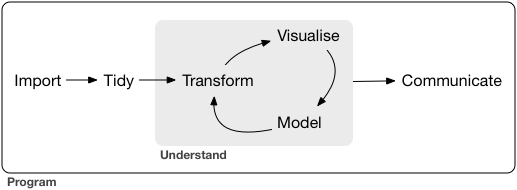
EDA is an iterative cycle. You:

Generate questions about your data.
Search for answers by visualising, transforming, and modelling your data.
Use what you learn to refine your questions and/or generate new questions.

“There are no routine statistical questions, only questionable statistical routines.” — Sir David Cox (1924-2022)

“Far better an approximate answer to the right question, which is often vague, than an exact answer to the wrong question, which can always be made precise.” — John Tukey (1915-2000)

6.1.2 Exploration in Visualization, II – r4ds:EDA

The very basic questions:

What type of variation occurs within my variables?
What type of covariation occurs between my variables?

Typical values

Which values are the most common? Why?
Which values are rare? Why? Does that match your expectations?
Can you see any unusual patterns? What might explain them?

6.1.3 Exploration in Visualization, III – r4ds:EDA

Clusters and Groups

How are the observations within each cluster similar to each other?
How are the observations in separate clusters different from each other?
How can you explain or describe the clusters?
Why might the appearance of clusters be misleading?

Outliers and Unusual Values

Sometimes outliers are data entry errors; other times outliers suggest important new science.

6.1.4 Exploration in Visualization, IV – r4ds:EDA

Patterns and models

Could this pattern be due to coincidence (i.e. random chance)?
How can you describe the relationship implied by the pattern?
How strong is the relationship implied by the pattern?
What other variables might affect the relationship?
Does the relationship change if you look at individual subgroups of the data?

6.1.5 EDA and Data Modeling: Simple Summary of Data

Goal: A simple low-dimensional summary of a dataset. Ideally, the model will capture true “signals” (i.e. patterns generated by the phenomenon of interest), and ignore “noise” (i.e. random variation that you’re not interested in).

“predictive” models: supervised
“data discovery” models: unsupervised

6.1.5.1 EDA (A diagram from R4DS by H.W. and G.G.)

EDA from r4ds

6.1.6 Hypothesis generation vs. hypothesis confirmation

Each observation can either be used for exploration or confirmation, not both.
You can use an observation as many times as you like for exploration, but you can only use it once for confirmation. As soon as you use an observation twice, you’ve switched from confirmation to exploration.

If you are serious about doing an confirmatory analysis, one approach is to split your data into three pieces before you begin the analysis:

60% of your data goes into a training (or exploration) set. You’re allowed to do anything you like with this data: visualise it and fit tons of models to it.
20% goes into a query set. You can use this data to compare models or visualisations by hand, but you’re not allowed to use it as part of an automated process.
20% is held back for a test set. You can only use this data ONCE, to test your final model.

6.1.7 R4DS: Model Basics

There are two parts to a model:

First, you define a family of models that express a precise, but generic, pattern that you want to capture. For example, the pattern might be a straight line, or a quadratic curve. You will express the model family as an equation like \(y = a_1 * x + a_2\) or \(y = a_1 * x ^ {a_2}\). Here, \(x\) and \(y\) are known variables from your data, and \(a_1\) and \(a_2\) are parameters that can vary to capture different patterns.
Next, you generate a fitted model by finding the model from the family that is the closest to your data. This takes the generic model family and makes it specific, like \(y = 3 * x + 7\) or \(y = 9 * x ^ 2\).

It’s important to understand that a fitted model is just the closest model from a family of models. That implies that you have the “best” model (according to some criteria); it doesn’t imply that you have a good model and it certainly doesn’t imply that the model is “true”.

6.1.8 All models are wrong, but some are useful. - George E.P. Box (1919-2013)

Now it would be very remarkable if any system existing in the real world could be exactly represented by any simple model. However, cunningly chosen parsimonious models often do provide remarkably useful approximations. For example, the law PV = RT relating pressure P, volume V and temperature T of an “ideal” gas via a constant R is not exactly true for any real gas, but it frequently provides a useful approximation and furthermore its structure is informative since it springs from a physical view of the behavior of gas molecules.

For such a model there is no need to ask the question “Is the model true?”. If “truth” is to be the “whole truth” the answer must be “No”. The only question of interest is “Is the model illuminating and useful?”.

The goal of a model is not to uncover truth, but to discover a simple approximation that is still useful.

6.1.9 Regression Analysis (wikipedia)

In statistical modeling, regression analysis is a set of statistical processes for estimating the relationships between a dependent variable (‘outcome variable’) and one or more independent variables (‘predictors’, ‘covariates’, or ‘features’). The most common form of regression analysis is linear regression, in which a researcher finds the line (or a more complex linear combination) that most closely fits the data according to a specific mathematical criterion.

Two purposes of regression analysis: First, regression analysis is widely used for prediction and forecasting. Second, regression analysis can be used to infer causal relationships between the independent and dependent variables. Importantly, regressions by themselves only reveal relationships between a dependent variable and a collection of independent variables in a fixed dataset. To use regressions for prediction or to infer causal relationships, respectively, a researcher must carefully justify why existing relationships have predictive power for a new context or why a relationship between two variables has a causal interpretation.

6.1.10 History of Regression Analysis (wikipedia)

The earliest form of regression was the method of least squares, which was published by Legendre in 1805, and by Gauss in 1809. Legendre and Gauss both applied the method to the problem of determining, from astronomical observations, the orbits of bodies about the Sun (mostly comets, but also later the then newly discovered minor planets). Gauss published a further development of the theory of least squares in 1821, including a version of the Gauss–Markov theorem.

The term “regression” was coined by Francis Galton in the nineteenth century to describe a biological phenomenon. The phenomenon was that the heights of descendants of tall ancestors tend to regress down towards a normal average (a phenomenon also known as regression toward the mean). For Galton, regression had only this biological meaning, but his work was later extended by Udny Yule and Karl Pearson to a more general statistical context.

6.1.11 The First Example

plot(cars)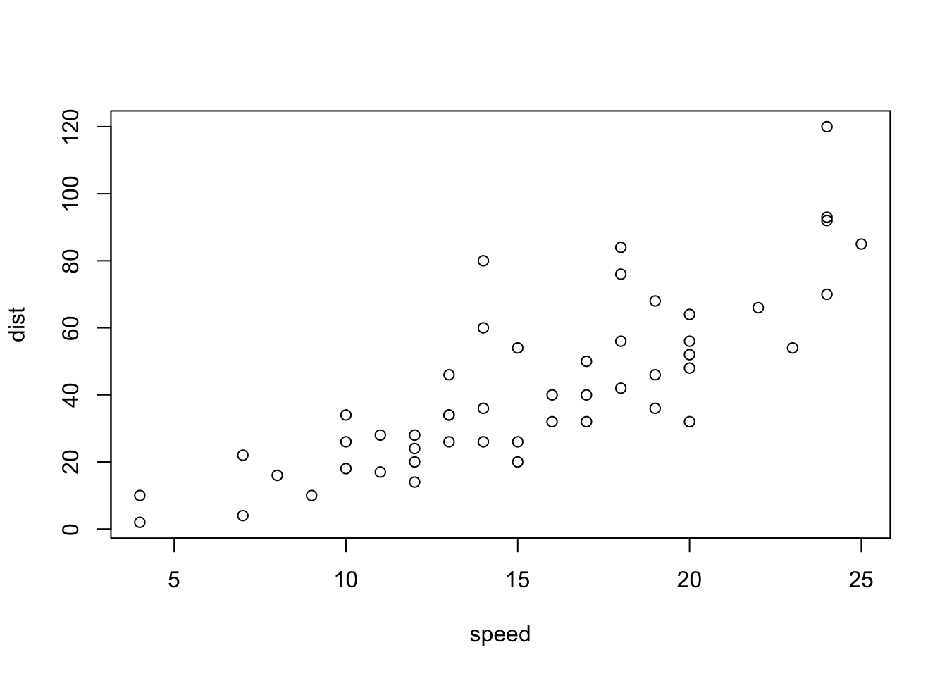

plot(cars) # cars: Speed and Stopping Distances of Cars
abline(lm(cars$dist~cars$speed))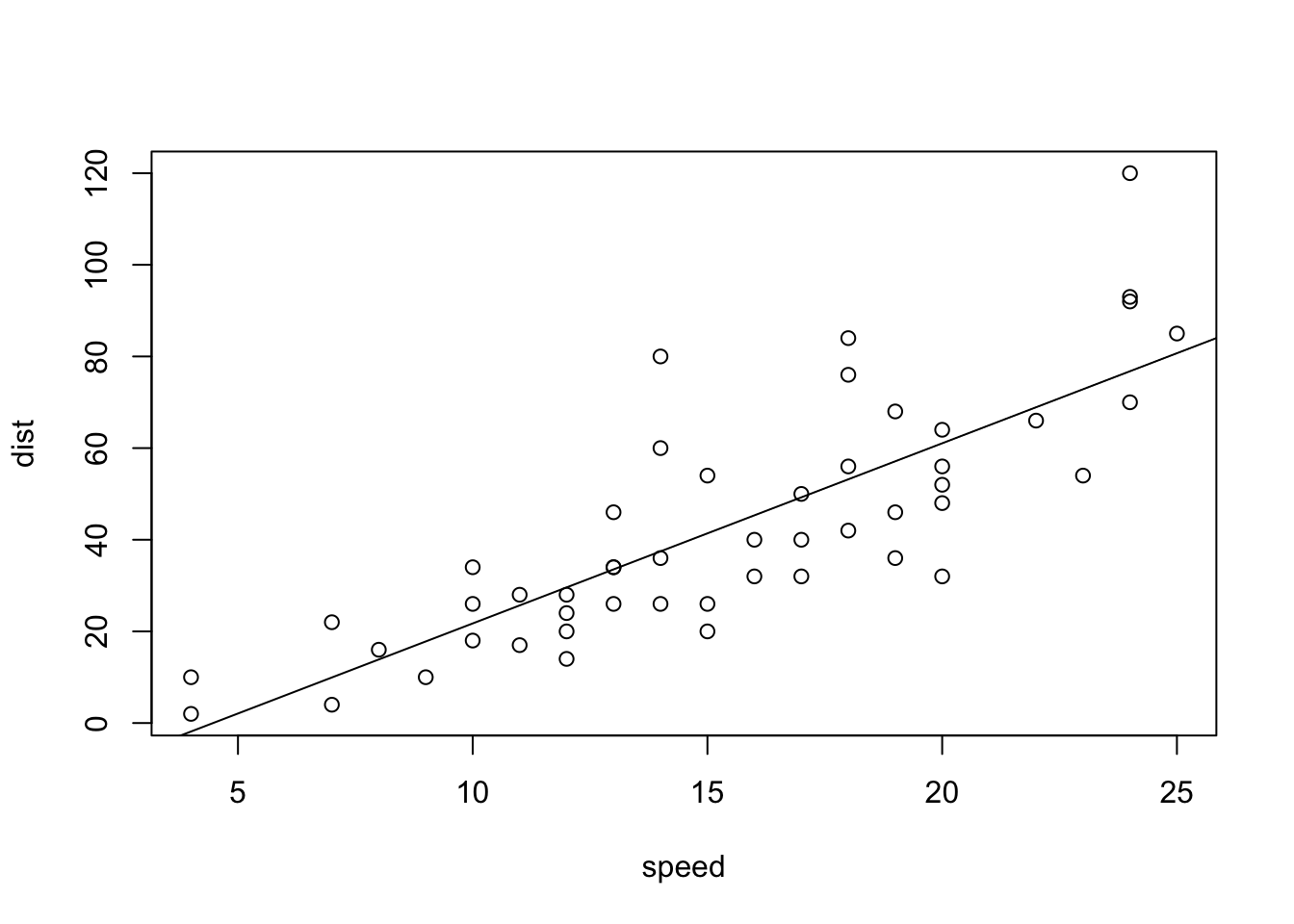

summary(lm(cars$dist~cars$speed))

## 
## Call:
## lm(formula = cars$dist ~ cars$speed)
## 
## Residuals:
##     Min      1Q  Median      3Q     Max 
## -29.069  -9.525  -2.272   9.215  43.201 
## 
## Coefficients:
##             Estimate Std. Error t value Pr(>|t|)    
## (Intercept) -17.5791     6.7584  -2.601   0.0123 *  
## cars$speed    3.9324     0.4155   9.464 1.49e-12 ***
## ---
## Signif. codes:  0 '***' 0.001 '**' 0.01 '*' 0.05 '.' 0.1 ' ' 1
## 
## Residual standard error: 15.38 on 48 degrees of freedom
## Multiple R-squared:  0.6511, Adjusted R-squared:  0.6438 
## F-statistic: 89.57 on 1 and 48 DF,  p-value: 1.49e-12

6.1.12 Model Analysis with `tidyverse`: `modelr`

Tidymodels: https://www.tidymodels.org
modelr: https://modelr.tidyverse.org
- Compute model quality for a given dataset

library(tidyverse)
library(modelr)
t_cars <- as_tibble(cars)
(mod <- lm(dist ~ speed, data = t_cars))

## 
## Call:
## lm(formula = dist ~ speed, data = t_cars)
## 
## Coefficients:
## (Intercept)        speed  
##     -17.579        3.932

## 
## Call:
## lm(formula = dist ~ speed, data = t_cars)
## 
## Residuals:
##     Min      1Q  Median      3Q     Max 
## -29.069  -9.525  -2.272   9.215  43.201 
## 
## Coefficients:
##             Estimate Std. Error t value Pr(>|t|)    
## (Intercept) -17.5791     6.7584  -2.601   0.0123 *  
## speed         3.9324     0.4155   9.464 1.49e-12 ***
## ---
## Signif. codes:  0 '***' 0.001 '**' 0.01 '*' 0.05 '.' 0.1 ' ' 1
## 
## Residual standard error: 15.38 on 48 degrees of freedom
## Multiple R-squared:  0.6511, Adjusted R-squared:  0.6438 
## F-statistic: 89.57 on 1 and 48 DF,  p-value: 1.49e-12

ggplot(t_cars, aes(speed, dist)) + geom_point() +
  geom_abline(slope = coef(mod)[[2]], intercept = coef(mod)[[1]])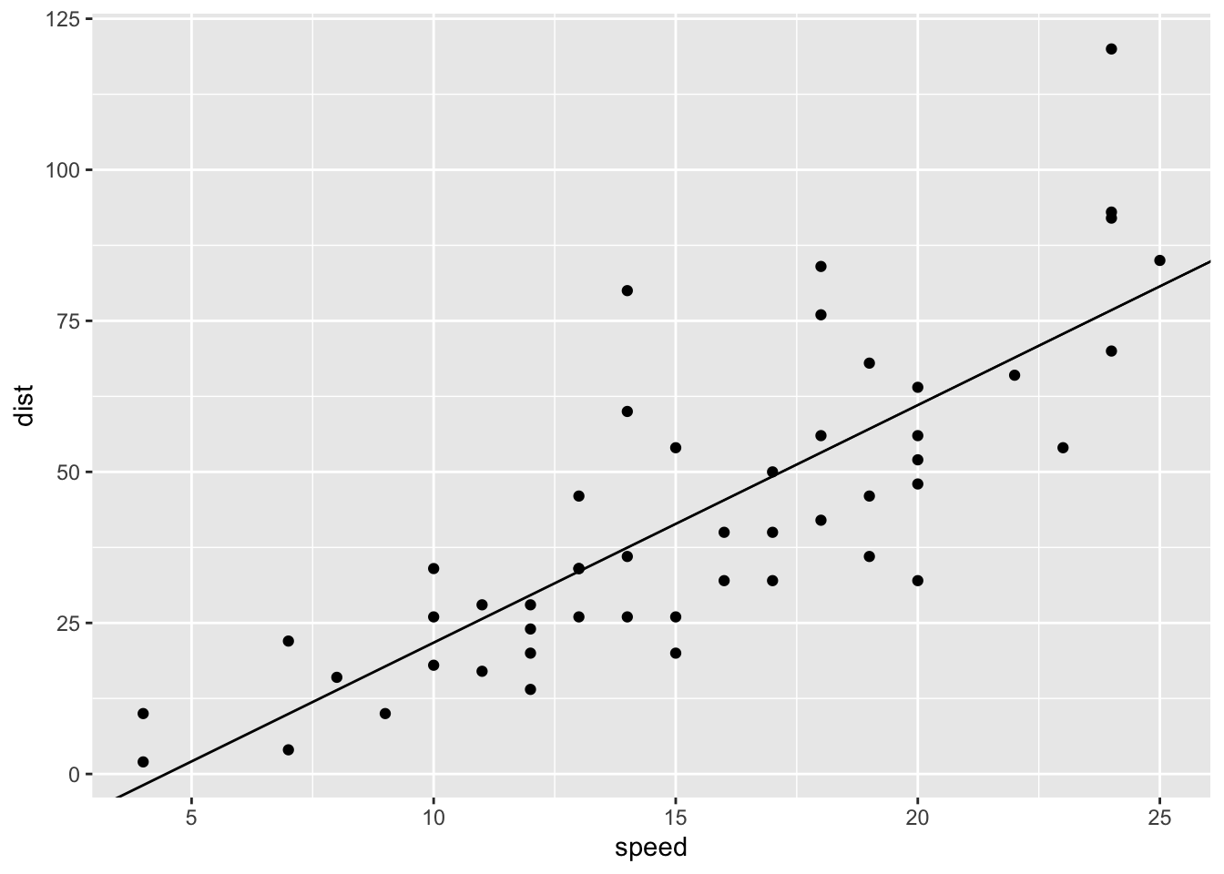

ggplot(t_cars, aes(speed, dist)) + geom_jitter() +
  geom_smooth(method = "lm", se = FALSE)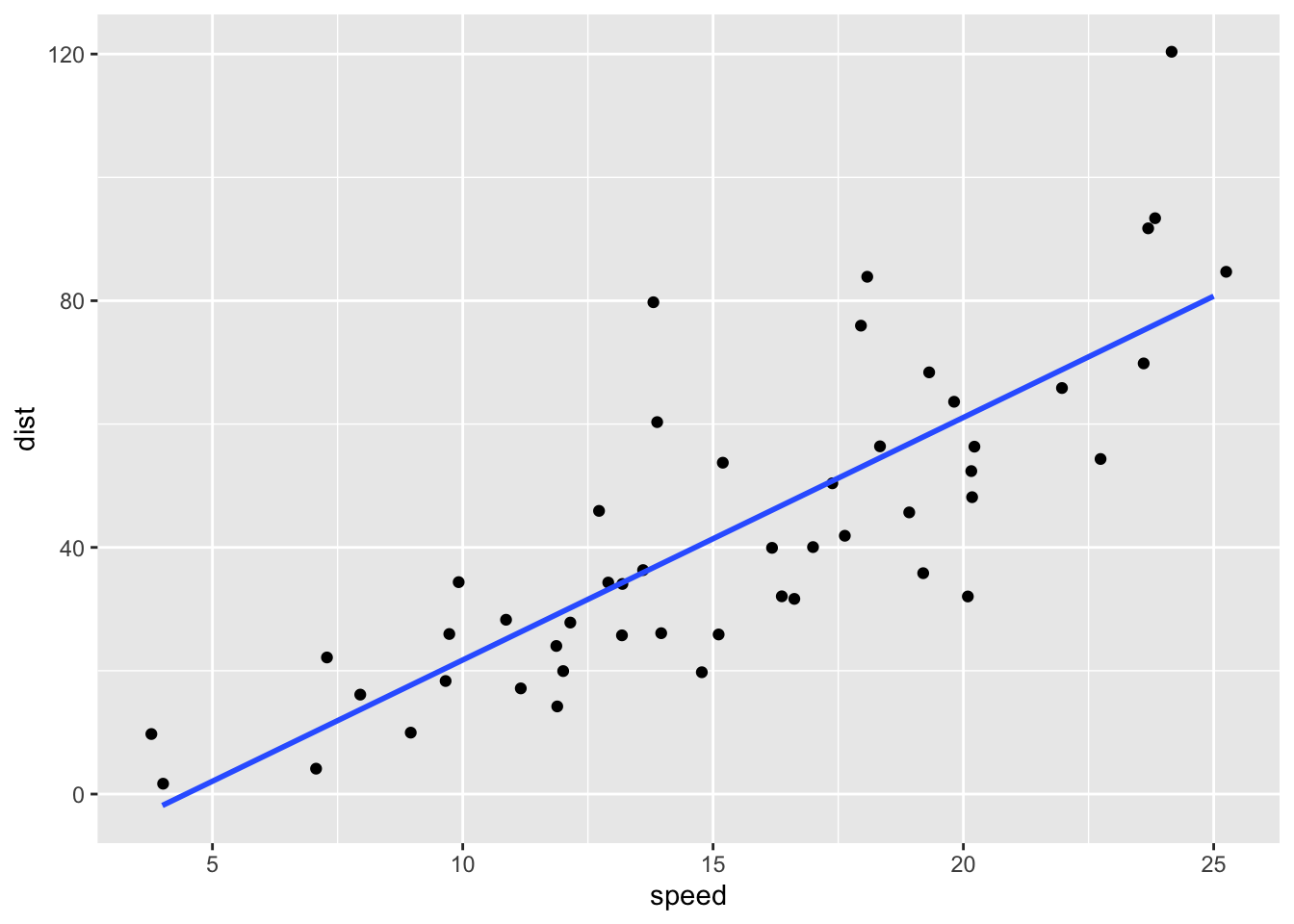

6.1.13 Predictions \(\hat{y} = a_1 + a_2x\) and Residuals \(y - \hat{y}\)

(mod_table <- t_cars %>% add_predictions(mod) %>% add_residuals(mod, var = "resid"))

## # A tibble: 50 × 4
##    speed  dist  pred resid
##    <dbl> <dbl> <dbl> <dbl>
##  1     4     2 -1.85  3.85
##  2     4    10 -1.85 11.8 
##  3     7     4  9.95 -5.95
##  4     7    22  9.95 12.1 
##  5     8    16 13.9   2.12
##  6     9    10 17.8  -7.81
##  7    10    18 21.7  -3.74
##  8    10    26 21.7   4.26
##  9    10    34 21.7  12.3 
## 10    11    17 25.7  -8.68
## # … with 40 more rows

mod_table %>% ggplot() + geom_jitter(aes(speed, resid)) + geom_hline(yintercept = 0)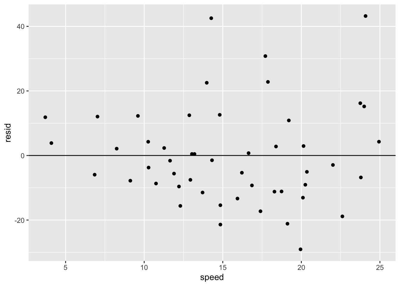

### geom_jitter()

t_cars %>% group_by(speed, dist) %>% 
  summarize(count = n()) %>% arrange(desc(count))

## `summarise()` has grouped output by 'speed'. You can override using the
## `.groups` argument.

## # A tibble: 49 × 3
## # Groups:   speed [19]
##    speed  dist count
##    <dbl> <dbl> <int>
##  1    13    34     2
##  2     4     2     1
##  3     4    10     1
##  4     7     4     1
##  5     7    22     1
##  6     8    16     1
##  7     9    10     1
##  8    10    18     1
##  9    10    26     1
## 10    10    34     1
## # … with 39 more rows

6.1.14 iris

(t_iris <- as_tibble(datasets::iris))

## # A tibble: 150 × 5
##    Sepal.Length Sepal.Width Petal.Length Petal.Width Species
##           <dbl>       <dbl>        <dbl>       <dbl> <fct>  
##  1          5.1         3.5          1.4         0.2 setosa 
##  2          4.9         3            1.4         0.2 setosa 
##  3          4.7         3.2          1.3         0.2 setosa 
##  4          4.6         3.1          1.5         0.2 setosa 
##  5          5           3.6          1.4         0.2 setosa 
##  6          5.4         3.9          1.7         0.4 setosa 
##  7          4.6         3.4          1.4         0.3 setosa 
##  8          5           3.4          1.5         0.2 setosa 
##  9          4.4         2.9          1.4         0.2 setosa 
## 10          4.9         3.1          1.5         0.1 setosa 
## # … with 140 more rows

6.1.15 Linear Model: Sepal.W ~ Sepal.L

colnames(t_iris) <- c("Sepal.L", "Sepal.W", "Petal.L", "Petal.W", "Species")

lm(Sepal.W ~ Sepal.L, data = t_iris)

## 
## Call:
## lm(formula = Sepal.W ~ Sepal.L, data = t_iris)
## 
## Coefficients:
## (Intercept)      Sepal.L  
##     3.41895     -0.06188

6.1.16 Linear Model: Petal.W ~ Petal.L

lm(Petal.W ~ Petal.L, data = t_iris)

## 
## Call:
## lm(formula = Petal.W ~ Petal.L, data = t_iris)
## 
## Coefficients:
## (Intercept)      Petal.L  
##     -0.3631       0.4158

6.1.17 Correlation

cor(t_iris[1:4])

##            Sepal.L    Sepal.W    Petal.L    Petal.W
## Sepal.L  1.0000000 -0.1175698  0.8717538  0.8179411
## Sepal.W -0.1175698  1.0000000 -0.4284401 -0.3661259
## Petal.L  0.8717538 -0.4284401  1.0000000  0.9628654
## Petal.W  0.8179411 -0.3661259  0.9628654  1.0000000

6.1.18 `filter(Species == "setosa")`

t_iris %>% filter(Species == "setosa") %>%
  ggplot(aes(x = Petal.L, y = Petal.W)) + 
  geom_point() + geom_smooth(method = "lm", se = FALSE)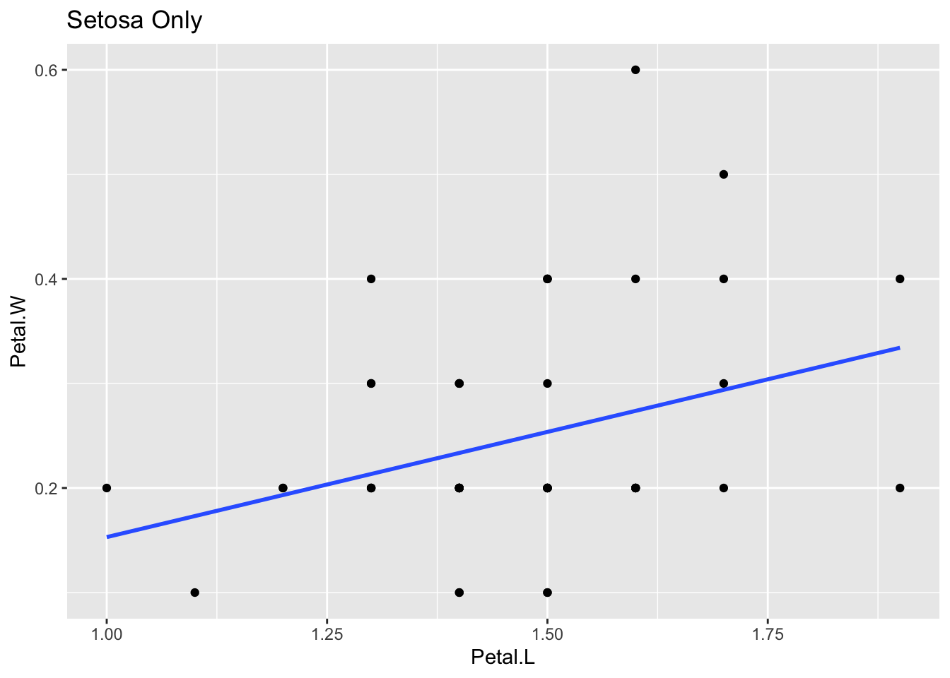

6.1.19 `aes(Sepal.L, Sepal.W, color = Species)`

6.1.20 Linear Regression Quick Reference

DataCamp:
- https://www.datacamp.com/community/tutorials/linear-regression-R
  1. What is a linear regression?
  2. Creating a linear regression in R.
  3. Learn the concepts of coefficients and residuals.
  4. How to test if your linear model has a good fit?
  5. Detecting influential points.
- DataCamp Top: https://www.datacamp.com - to be introduced
r-statistics.co by Selva Prabhakaran:
- http://r-statistics.co/Linear-Regression.html
  - The aim of linear regression is to model a continuous variable Y as a mathematical function of one or more X variable(s), so that we can use this regression model to predict the Y when only the X is known. This mathematical equation can be generalized as follows:
  - \(Y = \beta_1 + \beta_2 X + \varepsilon\)
- r-statistics.co Top: http://r-statistics.co
  - An educational resource for those seeking knowledge related to machine learning and statistical computing in R.

6.2 Part II: Practicum - Model Analysis Warnings

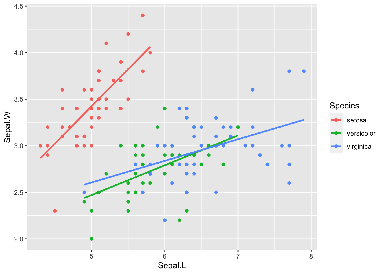
6.2.1 Linear Regression: `aes(Sepal.L, Sepal.W, color = Species)`

6.2.2 `aes(Sepal.L, Sepal.W, color = Species)`

## Warning: Using `size` aesthetic for lines was deprecated in ggplot2 3.4.0.
## ℹ Please use `linewidth` instead.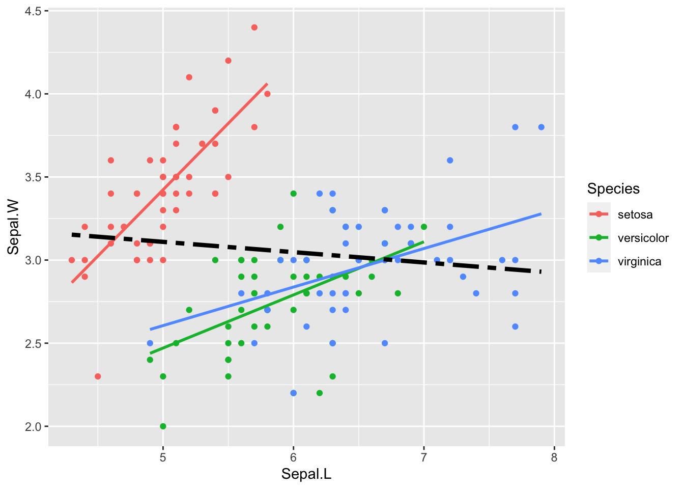

6.2.3 Correlation and Covariance

cor(t_iris[1:4])

##            Sepal.L    Sepal.W    Petal.L    Petal.W
## Sepal.L  1.0000000 -0.1175698  0.8717538  0.8179411
## Sepal.W -0.1175698  1.0000000 -0.4284401 -0.3661259
## Petal.L  0.8717538 -0.4284401  1.0000000  0.9628654
## Petal.W  0.8179411 -0.3661259  0.9628654  1.0000000

cov(t_iris[1:4])

##            Sepal.L    Sepal.W    Petal.L    Petal.W
## Sepal.L  0.6856935 -0.0424340  1.2743154  0.5162707
## Sepal.W -0.0424340  0.1899794 -0.3296564 -0.1216394
## Petal.L  1.2743154 -0.3296564  3.1162779  1.2956094
## Petal.W  0.5162707 -0.1216394  1.2956094  0.5810063

6.2.4 Useful Mathematical Formula

Let \(x = c(x_1, x_2, \ldots, x_n)\) be the independent variable, i.e., Sepal.L
Let \(y = c(y_1, y_2, \ldots, y_n)\) be the dependent variable, i.e., Sepal.W
Let \(\mbox{pred} = c(\hat{y}_1, \hat{y}_2, \ldots, \hat{y}_n)\) be the predicted values by linear regression. \[ \begin{aligned} \mbox{slope of the regression line} &= \frac{cov(x,y)}{var(x)} = \frac{cor(x,y)\sqrt{var(y)}}{\sqrt{var(x)}}\\ \mbox{total sum of squares} &= SS_{tot} = sum((y-mean(y))^2)\\ \mbox{residual sum of squares} &= SS_{res} = sum((y-\mbox{pred})^2)\\ \mbox{R squared} = R^2 & = 1 - \frac{SS_{res}}{SS_{tot}} = cor(x,y)^2 \end{aligned} \]

6.2.5 p-value

6.2.6 t-statistic

6.2.7 Mathematical Formulas, I

Let \(x = c(x_1, x_2, \ldots, x_n)\) be the independent variable, e.g., the height of fathers
Let \(y = c(y_1, y_2, \ldots, y_n)\) be the dependent variable, i.e., height of children
Let \(\mbox{pred} = c(\hat{y}_1, \hat{y}_2, \ldots, \hat{y}_n)\) be the predicted values by linear regression.

6.2.8 Mathematical Formulas, II

\[ \begin{aligned} \mbox{unbiased covariance: } cov(x,y) &= \frac{\sum_{i=1}^n(x_i - mean(x))(y_i - mean(y))}{n-1}\\ \mbox{unviased variance: } var(x) &= cov(x,x) \\ \mbox{correlation: } cor(x.y) &= \frac{cov(x,y)}{\sqrt{var(x)var(y)}}\\ \mbox{slope of the regression line} &= \frac{cov(x,y)}{var(x)} = \frac{cor(x,y)\sqrt{var(y)}}{\sqrt{var(x)}}\\ \mbox{total sum of squares} &= SS_{tot} = \sum_{i=1}^n((y_i-mean(y))^2)\\ \mbox{residual sum of squares} &= SS_{res} = \sum_{i=1}^n((y_i-\hat{y}_i)^2)\\ \mbox{R squared} = R^2 & = 1 - \frac{SS_{res}}{SS_{tot}} = cor(x,y)^2 \end{aligned} \]

6.2.9 Regression Analyais: Summary

R-Squared: Higher the better (> 0.70)
- How well the prediction fit to the data. \(0 \leq R2 \leq 1\).
- For linear regression between two variables x and y, R-squared is the square of cor(x,y).
- R-Squared can be measured on any prediction model.
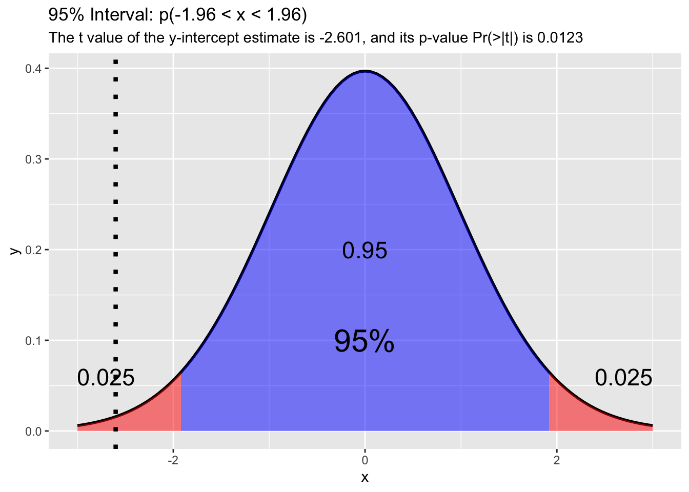
t-statistic: The absolute value should be greater 1.96, and for p-value be less than 0.05
- The model and the choice of variable(s) are suitable or not.
- p-value appears in Hypothesis testing (A/B test, sensitivity - specificity, etc.)

6.2.10 The ASA Statement on p-Values: Context, Process, and Purpose

P-values can indicate how incompatible the data are with a specified statistical model.
P-values do not measure the probability that the studied hypothesis is true, or the probability that the data were produced by random chance alone.
Scientific conclusions and business or policy decisions should not be based only on whether a p-value passes a specific threshold.
Proper inference requires full reporting and transparency.
A p-value, or statistical significance, does not measure the size of an effect or the importance of a result.
By itself, a p-value does not provide a good measure of evidence regarding a model or hypothesis.

AMERICAN STATISTICAL ASSOCIATION RELEASES STATEMENT ON STATISTICAL SIGNIFICANCE AND P-VALUES

6.2.11 Public Data: UN Data and US Census

UN Data: https://data.un.org
Uited States Census Bureau: https://www.census.gov

6.2.11.1 Importing Data

Get the URL (uniform resource locator) - copy the link

url_of_data <- "https://data.un.org/--long url--.csv"

Download the file into the destfile in data folder:

download.file(url = url_of_data, destfile = "data/un_pop.csv")

Read the file:

df_un_pop <- read_csv("data/un_pop.csv")

6.2.12 An Example: US Census Bureau

International Data Base (IDB)
idbzip.zip is a large archive with three files; idb5yr.all, idbsingleyear.all and Readme.txt. The data of idbsingleyear.all is separated by | and contains over 3 million rows.
Execute the following code only once. Then commnet these lines out with #.

6.2.12.1 Importance of Population Data of Each Country

Population: Special meaning in statistics
- In statistics, a population is a set of similar items or events which is of interest for some question or experiment.
Basis of analysis
Public Opinion Poll

6.2.13 OECD: About Who we are

The Organisation for Economic Co-operation and Development (OECD) is an international organisation that works to build better policies for better lives. Our goal is to shape policies that foster prosperity, equality, opportunity and well-being for all.

6.2.13.1 Data

http://www.oecd.org
Data: https://data.oecd.org
OECD.Stat: https://stats.oecd.org
- OECD.Stat Web Browser User Guide, May 2013
1. Search Box > Filter by type, Filter by topic, Sort results
2. Browse by Topic: Agriculture, Development, Economy, Education, Energy, Finance, Govetnment, Health, Innovation and Technology, Job, Society
3. Browse by Country: choose from 43 countries
4. Catalogue of OECD databases
5. Featured Charts, Latest News, Statistical Resources

6.2.14 Learning Resources, V

R for Data Science, Part IV Model

6.2.14.1 RStudio Primers: See References in Moodle at the bottom

The Basics – r4ds: Explore, I
Work with Data – r4ds: Wrangle, I
Visualize Data – r4ds: Explore, II

Exploratory Data Analysis, Bar Charts, Histograms
Boxplots and Counts, Scatterplots, Line Plots
Overplotting and Big Data, Customize Your Plots

Tidy Your Data – r4ds: Wrangle, II

Reshape Data, Separate and Unite Columns, Join Data Sets

6.2.15 Learning Resources – Summary

Books
- Textbook: R for Data Science
- Books Online: BOOKDOWN
Exercise Tools
- {swirl} Learn R in R
- R Studio Cloud Primers
Others
- R Studio Education
- Cheat Sheet

Data Science is an empirical study! Develop your skills and knowledge by experiences.

Data Science is for Everyone!

6.3 The Sixth Assignment (in Moodle)

Choose a public data. Clearly state how you obtained the data. Even if you are able to give the URL to download the data, explain the steps you reached and obtained the data.
Create an R Notebook (file name.nb.html, e.g. a6_12345.nb.html) of an EDA containing:
1. title, date, and author, i.e., Your Name
2. your motivation and/or objectives to analyze the data, and your questions
3. an explanation of the data and the variables
4. chunks containing the following:
  - library(tidyverse, modelr),
  - visualization of the data with ggplot()
  - both a linear model (summary(lm(y~x))) and a chart created by ggplot() with fitted line.
5. explanation of the values given by the model and describe a prediction or a finding using the model.
6. your findings and/or questions
Submit your R Notebook file to Moodle (The Sixth Assignment) by 2021-02-01 23:59:00

6.3.1 Setup and YAML

This R Notebook document uses the following YAML:

---
title: "Responses to the Sixth Assignment on Modeling and EDA"
author: "p000117x Hiroshi Suzuki"
date: '2022-02-07'
output: 
  html_notebook:
    number_sections: yes
    toc: yes
    toc_float: yes
---

6.3.2 Packages to load

https://tidyverse.tidyverse.org/

library(tidyverse) will load the core tidyverse packages:

ggplot2, for data visualisation.
dplyr, for data manipulation.
tidyr, for data tidying.
readr, for data import.
purrr, for functional programming.
tibble, for tibbles, a modern re-imagining of data frames.
stringr, for strings.
forcats, for factors.

Hence the following code chunk loads every core package above, and modelr. Although modelr is a tidyverse package but it is not a core tidyverse package, you need to add library(modelr).

library(tidyverse)
library(modelr)

We will use WDI package for examples.

library(WDI)

6.3.3 Modeling and EDA Summary

Reference: * r4ds:EDA * R4DS: Model Basics

Importing
Glimpsing
Transforming
Visualising
Modeling

6.3.3.1 Exploration in Visualization

EDA is an iterative cycle. You:

Generate questions about your data.
Search for answers by visualising, transforming, and modelling your data. - Methods in Data Science
Use what you learn to refine your questions and/or generate new questions.

“There are no routine statistical questions, only questionable statistical routines.” — Sir David Cox (1924.7.15-2022.1.18)

“Far better an approximate answer to the right question, which is often vague, than an exact answer to the wrong question, which can always be made precise.” — John Tukey (1915.6.16-2000.7.26)

Exploratory Data Analysis cannot be done by statistical routines or a list of routine questions.

6.3.3.2 Quotation Marks

Reference: https://stat.ethz.ch/R-manual/R-devel/library/base/html/Quotes.html

Three types of quotes are part of the syntax of R: single and double quotation marks and the backtick (or back quote, ‘⁠`⁠’). Backslash is used to start an escape sequence inside character constants.

Single and double quotes delimit character constants. They can be used interchangeably but double quotes are preferred (and character constants are printed using double quotes), so single quotes are normally only used to delimit character constants containing double quotes.
‘single quotes can be used more-or-less interchangeably’
“with double quotes to create character vectors”

identical('"It\'s alive!", he screamed.',
          "\"It's alive!\", he screamed.") # same

## [1] TRUE

Backticks are used for non-standard variable names. (See make.names and ?Reserved for what counts as non-standard.)
- When you have a space, or other special characters, in the variable name, use backticks.

`x y` <- 1:5  # variable
`x y`         # variable

## [1] 1 2 3 4 5

"x y" <- 1:5  # variable
`x y`         # variable

## [1] 1 2 3 4 5

"x y"         # character vector

## [1] "x y"

d <- data.frame(`1st column` = rchisq(5, 2), check.names = FALSE)
d$`1st column`

## [1] 1.51940165 0.91352143 0.17061561 0.01771576 1.31073623

6.3.4 Examples and Comments

6.3.4.1 Preparations

6.3.4.1.1 Extra Packages

In the following we use modelsummary which Prof Kaizoji introduced at his Week 7 lecture. You need to install it if you have not by the followiin in you console or from Tools menu on top.

See: https://CRAN.R-project.org/package=modelsummary

install.packages("modelsummary")

library(modelsummary) # Tool for writting tables of the regression results

6.3.5 CLASS.xlsx

See Responses to Assignment Five.

6.3.5.1 Importing Excel Files

CLASS.xlsx: - copy the following link
- The current classification by income in XLS format
readxl: https://readxl.tidyverse.org
Help: read_excel, read_xls, read_xlsx

url_class <- "https://databankfiles.worldbank.org/data/download/site-content/CLASS.xlsx"
download.file(url = url_class, destfile = "data/CLASS.xlsx")

6.3.5.1.1 Countries

Let us look at the first sheet.

The column names are in the 5th row.
The country data starts from the 7th row.
Zimbabue is at the last row.

library(readxl)
wb_countries_tmp <- read_excel("data/CLASS.xlsx", sheet = 1, skip = 0, n_max =219) 
wb_countries <- wb_countries_tmp %>% 
  select(country = Economy, iso3c = Code, region = Region, income = `Income group`, lending = "Lending category", other = "Other (EMU or HIPC)")
wb_countries

## # A tibble: 218 × 6
##    country              iso3c region                     income    lending other
##    <chr>                <chr> <chr>                      <chr>     <chr>   <chr>
##  1 Aruba                ABW   Latin America & Caribbean  High inc… <NA>    <NA> 
##  2 Afghanistan          AFG   South Asia                 Low inco… IDA     HIPC 
##  3 Angola               AGO   Sub-Saharan Africa         Lower mi… IBRD    <NA> 
##  4 Albania              ALB   Europe & Central Asia      Upper mi… IBRD    <NA> 
##  5 Andorra              AND   Europe & Central Asia      High inc… <NA>    <NA> 
##  6 United Arab Emirates ARE   Middle East & North Africa High inc… <NA>    <NA> 
##  7 Argentina            ARG   Latin America & Caribbean  Upper mi… IBRD    <NA> 
##  8 Armenia              ARM   Europe & Central Asia      Upper mi… IBRD    <NA> 
##  9 American Samoa       ASM   East Asia & Pacific        Upper mi… <NA>    <NA> 
## 10 Antigua and Barbuda  ATG   Latin America & Caribbean  High inc… IBRD    <NA> 
## # … with 208 more rows

6.3.5.1.2 Regions

readxl: https://readxl.tidyverse.org
Help: read_excel, read_xls, read_xlsx

Regions start from the 221th row.
Regions end at the 266th row.

wb_regions_tmp <- read_excel("data/CLASS.xlsx", sheet = 1, skip = 0, n_max =266) %>% 
  slice(-(1:220))
wb_regions <- wb_regions_tmp %>% 
  select(region = Economy, iso3c = Code) %>% drop_na()
wb_regions

## # A tibble: 45 × 2
##    region                                        iso3c
##    <chr>                                         <chr>
##  1 Caribbean small states                        CSS  
##  2 Central Europe and the Baltics                CEB  
##  3 Early-demographic dividend                    EAR  
##  4 East Asia & Pacific                           EAS  
##  5 East Asia & Pacific (excluding high income)   EAP  
##  6 East Asia & Pacific (IDA & IBRD)              TEA  
##  7 Euro area                                     EMU  
##  8 Europe & Central Asia                         ECS  
##  9 Europe & Central Asia (excluding high income) ECA  
## 10 Europe & Central Asia (IDA & IBRD)            TEC  
## # … with 35 more rows

Let us look at the second sheet.

wb_groups_tmp <- read_excel("data/CLASS.xlsx", sheet = "Groups") # sheet = 3
wb_groups <- wb_groups_tmp %>% 
  select(gcode = GroupCode, group = GroupName, iso3c = CountryCode, country = CountryName)

6.3.6 Population and GDP per Capita

6.3.6.1 Importing

WDIsearch(string = "SP.POP.TOTL", field = "indicator")

##                indicator                                             name
## 17674        SP.POP.TOTL                                Population, total
## 17675  SP.POP.TOTL.FE.IN                               Population, female
## 17676  SP.POP.TOTL.FE.ZS       Population, female (% of total population)
## 17677    SP.POP.TOTL.ICP                       SP.POP.TOTL.ICP:Population
## 17678 SP.POP.TOTL.ICP.ZS SP.POP.TOTL.ICP.ZS:Population shares (World=100)
## 17679  SP.POP.TOTL.MA.IN                                 Population, male
## 17680  SP.POP.TOTL.MA.ZS         Population, male (% of total population)
## 17681     SP.POP.TOTL.ZS                          Population (% of total)

df_pop_gdpcap <- WDI(
  country = "all",
  indicator = c(pop ="SP.POP.TOTL", gdpcap = "NY.GDP.PCAP.KD"),
  start = 1961,
  end = 2020
)
head(df_pop_gdpcap)

##       country iso2c iso3c year      pop gdpcap
## 1 Afghanistan    AF   AFG 1961  9169406     NA
## 2 Afghanistan    AF   AFG 1962  9351442     NA
## 3 Afghanistan    AF   AFG 1963  9543200     NA
## 4 Afghanistan    AF   AFG 1964  9744772     NA
## 5 Afghanistan    AF   AFG 1965  9956318     NA
## 6 Afghanistan    AF   AFG 1966 10174840     NA

6.3.6.2 Visializing and Modeling

df_pop_gdpcap %>% filter(country == "World") %>% 
  ggplot(aes(x = pop, y = gdpcap)) + geom_point() + geom_smooth(method = "lm", se = FALSE)

## `geom_smooth()` using formula = 'y ~ x'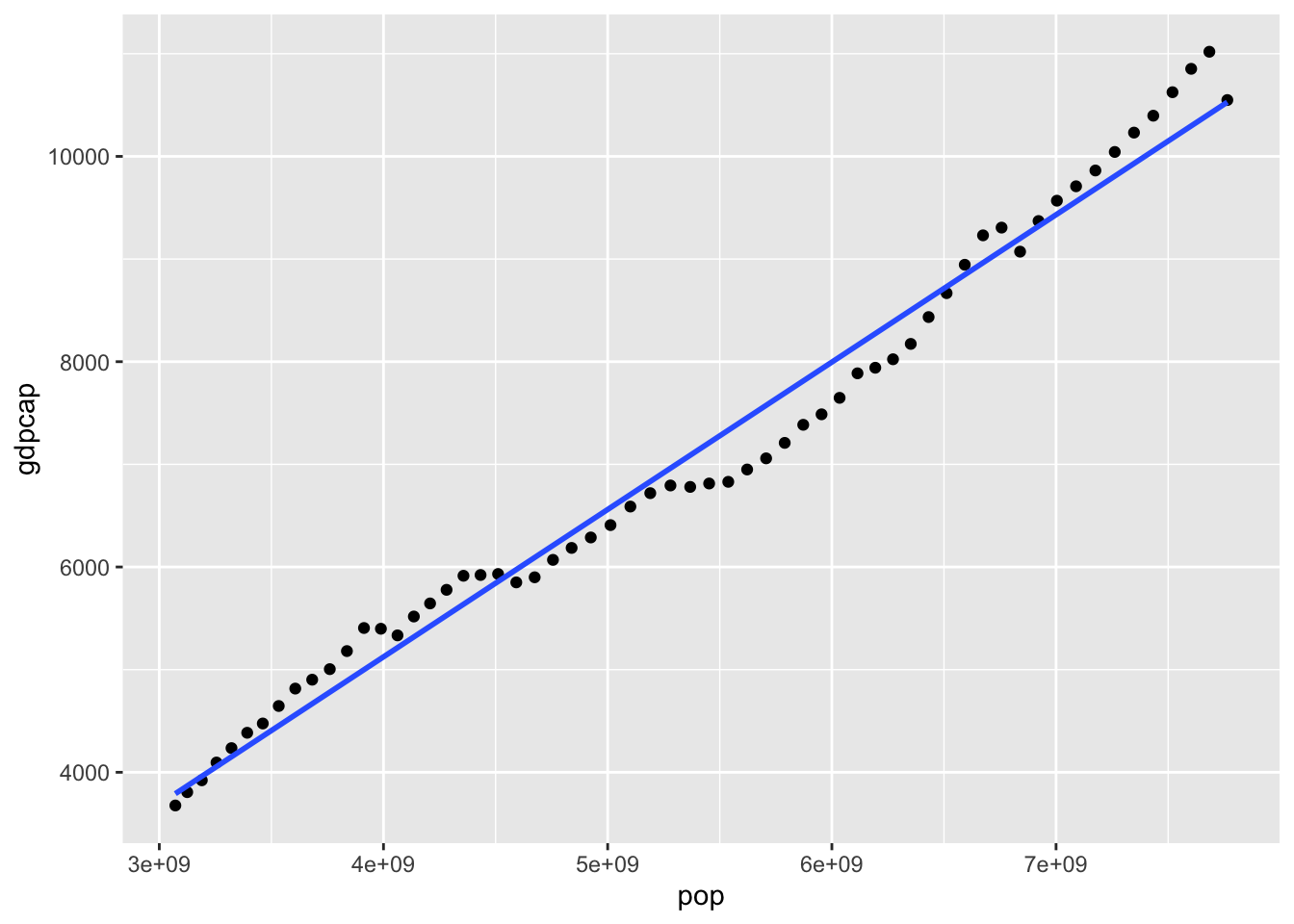

df_pop_gdpcap %>% filter(country == "World") -> df_pk
df_pk %>% lm(gdpcap ~ pop, .) %>% summary()

## 
## Call:
## lm(formula = gdpcap ~ pop, data = .)
## 
## Residuals:
##     Min      1Q  Median      3Q     Max 
## -516.54 -172.78   45.57  223.68  606.04 
## 
## Coefficients:
##               Estimate Std. Error t value Pr(>|t|)    
## (Intercept) -6.184e+02  1.447e+02  -4.272 7.28e-05 ***
## pop          1.436e-06  2.622e-08  54.759  < 2e-16 ***
## ---
## Signif. codes:  0 '***' 0.001 '**' 0.01 '*' 0.05 '.' 0.1 ' ' 1
## 
## Residual standard error: 284.8 on 58 degrees of freedom
## Multiple R-squared:  0.981,  Adjusted R-squared:  0.9807 
## F-statistic:  2999 on 1 and 58 DF,  p-value: < 2.2e-16

6.3.7 Internet

6.3.7.1 Importing

df_un_internet <- read_csv("https://data.un.org/_Docs/SYB/CSV/SYB64_314_202110_Internet%20Usage.csv", skip = 1)

## New names:
## Rows: 1357 Columns: 7
## ── Column specification
## ──────────────────────────────────────────────────────────────────────────────────────────────────────
## Delimiter: "," chr (4): ...2, Series, Footnotes, Source dbl (3): Region/Country/Area, Year, Value
## ℹ Use `spec()` to retrieve the full column specification for this data. ℹ Specify the column types or set `show_col_types =
## FALSE` to quiet this message.
## • `` -> `...2`

6.3.7.2 Glimpsing

We first overview the structure of the data briefly

head(df_un_internet)

## # A tibble: 6 × 7
##   `Region/Country/Area` ...2                    Year Series Value Footn…¹ Source
##                   <dbl> <chr>                  <dbl> <chr>  <dbl> <chr>   <chr> 
## 1                     1 Total, all countries …  2000 Perce…   6.5 <NA>    Inter…
## 2                     1 Total, all countries …  2005 Perce…  16.8 <NA>    Inter…
## 3                     1 Total, all countries …  2010 Perce…  29.3 <NA>    Inter…
## 4                     1 Total, all countries …  2015 Perce…  41.1 <NA>    Inter…
## 5                     1 Total, all countries …  2017 Perce…  46.3 <NA>    Inter…
## 6                     1 Total, all countries …  2018 Perce…  49   <NA>    Inter…
## # … with abbreviated variable name ¹Footnotes

glimpse(df_un_internet)

## Rows: 1,357
## Columns: 7
## $ `Region/Country/Area` <dbl> 1, 1, 1, 1, 1, 1, 1, 15, 15, 15, 15, 15, 15, 15,…
## $ ...2                  <chr> "Total, all countries or areas", "Total, all cou…
## $ Year                  <dbl> 2000, 2005, 2010, 2015, 2017, 2018, 2019, 2000, …
## $ Series                <chr> "Percentage of individuals using the internet", …
## $ Value                 <dbl> 6.5, 16.8, 29.3, 41.1, 46.3, 49.0, 51.4, 0.6, 9.…
## $ Footnotes             <chr> NA, NA, NA, NA, NA, NA, NA, NA, NA, NA, NA, NA, …
## $ Source                <chr> "International Telecommunication Union (ITU), Ge…

Note that the first column name is surrounded by backticks.

df_un_internet %>% summary()

##  Region/Country/Area     ...2                Year         Series         
##  Min.   :  1         Length:1357        Min.   :2000   Length:1357       
##  1st Qu.:156         Class :character   1st Qu.:2005   Class :character  
##  Median :388         Mode  :character   Median :2010   Mode  :character  
##  Mean   :393                            Mean   :2011                     
##  3rd Qu.:620                            3rd Qu.:2017                     
##  Max.   :894                            Max.   :2019                     
##      Value        Footnotes            Source         
##  Min.   : 0.00   Length:1357        Length:1357       
##  1st Qu.: 8.00   Class :character   Class :character  
##  Median :34.10   Mode  :character   Mode  :character  
##  Mean   :39.01                                        
##  3rd Qu.:68.10                                        
##  Max.   :99.70

df_un_internet %>% distinct(Source)

## # A tibble: 1 × 1
##   Source                                                                        
##   <chr>                                                                         
## 1 International Telecommunication Union (ITU), Geneva, the ITU database, last a…

All sources are ‘International Telecommunication Union (ITU), Geneva, the ITU database, last accessed January 2021’.

df_un_internet %>% distinct(Footnotes)

## # A tibble: 71 × 1
##    Footnotes                                                                    
##    <chr>                                                                        
##  1 <NA>                                                                         
##  2 Estimate.                                                                    
##  3 Population aged 15 years and over.                                           
##  4 Population aged 15 years and over.;Accessed the internet for personal use in…
##  5 Population aged 14 years and over.                                           
##  6 Population aged 16 to 74 years.                                              
##  7 Population aged 16 to 74 years.;Users in the last 3 months.                  
##  8 Population aged 7 years and over.                                            
##  9 Population aged 16 years and over.                                           
## 10 Users in the last 12 months.                                                 
## # … with 61 more rows

df_un_internet %>% distinct(Series)

## # A tibble: 1 × 1
##   Series                                      
##   <chr>                                       
## 1 Percentage of individuals using the internet

There is only one series. ‘Percentage of individuals using the internet’ can be for the title.

df_un_internet %>% group_by(Footnotes) %>% summarize(number_of_regions = n_distinct(`...2`)) %>%
  arrange(desc(number_of_regions))

## # A tibble: 71 × 2
##    Footnotes                                                   number_of_regions
##    <chr>                                                                   <int>
##  1 <NA>                                                                      236
##  2 Estimate.                                                                 151
##  3 Population aged 16 to 74 years.                                            31
##  4 Users in the last 3 months.                                                16
##  5 Population aged 5 years and over.                                           9
##  6 Population aged 6 years and over.                                           9
##  7 Estimate.;Population aged 18 years and over.                                8
##  8 Population aged 15 years and over.                                          6
##  9 Population aged 16 to 74 years.;Users in the last 3 months.                 6
## 10 Population aged 10 years and over.                                          5
## # … with 61 more rows

We need to see Footnotes carefully but in the beginning we do not examine.

df_un_internet %>% distinct(Year)

## # A tibble: 7 × 1
##    Year
##   <dbl>
## 1  2000
## 2  2005
## 3  2010
## 4  2015
## 5  2017
## 6  2018
## 7  2019

df_un_internet %>% group_by(Year) %>% summarize(number_of_regions = n_distinct(...2)) %>%
  arrange(desc(number_of_regions))

## # A tibble: 7 × 2
##    Year number_of_regions
##   <dbl>             <int>
## 1  2010               233
## 2  2000               232
## 3  2005               232
## 4  2015               227
## 5  2017               222
## 6  2018               110
## 7  2019               101

df_un_internet %>% group_by(...2) %>% summarize(number_of_years = n_distinct(Year)) %>%
  arrange(number_of_years)

## # A tibble: 246 × 2
##    ...2                     number_of_years
##    <chr>                              <int>
##  1 "Cura\xe7ao"                           1
##  2 "Mayotte"                              1
##  3 "Montserrat"                           1
##  4 "Nauru"                                1
##  5 "Ascension"                            2
##  6 "British Virgin Islands"               2
##  7 "French Guiana"                        2
##  8 "Guadeloupe"                           2
##  9 "Guernsey"                             2
## 10 "Jersey"                               2
## # … with 236 more rows

df_un_internet %>% group_by(`Region/Country/Area`) %>% summarize(number_of_years = n_distinct(Year)) %>%
  arrange(number_of_years)

## # A tibble: 246 × 2
##    `Region/Country/Area` number_of_years
##                    <dbl>           <int>
##  1                   175               1
##  2                   500               1
##  3                   520               1
##  4                   531               1
##  5                    92               2
##  6                   254               2
##  7                   312               2
##  8                   412               2
##  9                   474               2
## 10                   638               2
## # … with 236 more rows

df_un_internet %>% distinct(`Region/Country/Area`, ...2)

## # A tibble: 246 × 2
##    `Region/Country/Area` ...2                         
##                    <dbl> <chr>                        
##  1                     1 Total, all countries or areas
##  2                    15 Northern Africa              
##  3                   202 Sub-Saharan Africa           
##  4                    14 Eastern Africa               
##  5                    17 Middle Africa                
##  6                    18 Southern Africa              
##  7                    11 Western Africa               
##  8                    21 Northern America             
##  9                   419 Latin America & the Caribbean
## 10                    29 Caribbean                    
## # … with 236 more rows

Region/Country/Area and names in …2 are in one to one correspondence. It seems that the first 21 of them are areas and data are aggregated and the rest of them are countries or regions.
Since these 21 regions are overlapping, we need to study the definition. Let us choose

area_num_tmp <- c(15, 202, 21, 29, 420, 142, 150, 9)

6.3.7.3 Transforming

df_internet <- df_un_internet %>%
  select(num = `Region/Country/Area`, region = ...2, year = Year, value = Value) %>%
  mutate(year = as.integer(year))
head(df_internet)

## # A tibble: 6 × 4
##     num region                         year value
##   <dbl> <chr>                         <int> <dbl>
## 1     1 Total, all countries or areas  2000   6.5
## 2     1 Total, all countries or areas  2005  16.8
## 3     1 Total, all countries or areas  2010  29.3
## 4     1 Total, all countries or areas  2015  41.1
## 5     1 Total, all countries or areas  2017  46.3
## 6     1 Total, all countries or areas  2018  49

area_vector <- df_internet %>% distinct(region) %>% slice(1:21) %>% pull()
area_vector

##  [1] "Total, all countries or areas" "Northern Africa"              
##  [3] "Sub-Saharan Africa"            "Eastern Africa"               
##  [5] "Middle Africa"                 "Southern Africa"              
##  [7] "Western Africa"                "Northern America"             
##  [9] "Latin America & the Caribbean" "Caribbean"                    
## [11] "Latin America"                 "Asia"                         
## [13] "Central Asia"                  "Eastern Asia"                 
## [15] "South-central Asia"            "South-eastern Asia"           
## [17] "Southern Asia"                 "Western Asia"                 
## [19] "Europe"                        "Oceania"                      
## [21] "Australia and New Zealand"

6.3.7.4 Visualising

df_internet %>% filter(region == "Total, all countries or areas") %>%
  ggplot(aes(x = year, y = value)) + geom_point() + geom_line()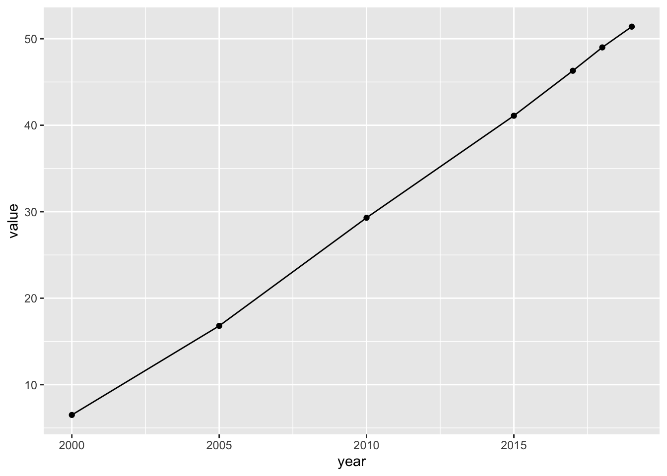

The value, ‘Percentage of individuals using the internet’ is increasing and almost on a straight line. We will study linear regression later.

df_internet %>% filter(num %in% area_num_tmp) %>%
  ggplot(aes(x = year, y = value, color = region)) + geom_line() + geom_point()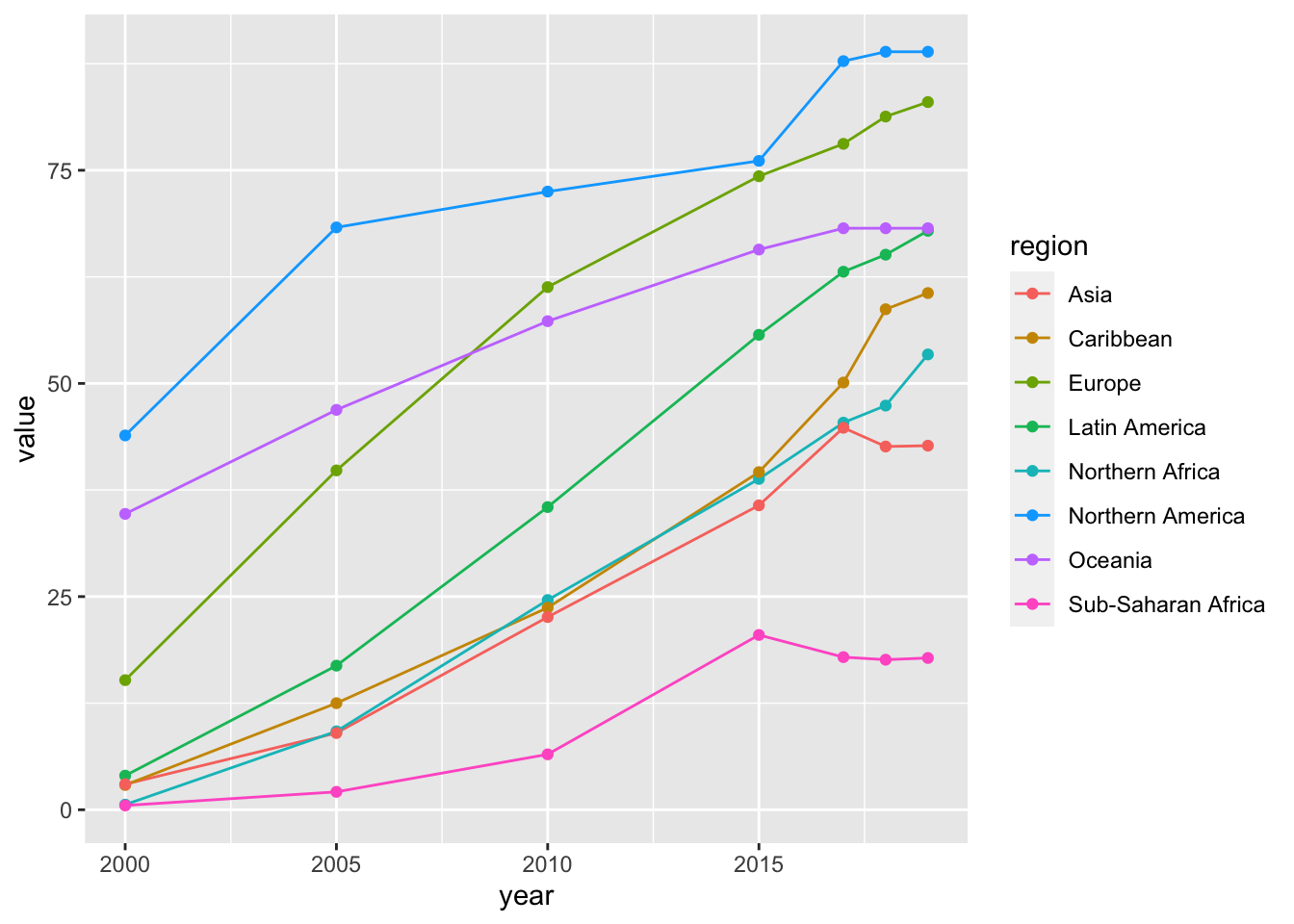

df_internet %>% filter(region %in% area_vector) %>%
  ggplot(aes(x = year, y = value, color = region)) + geom_line()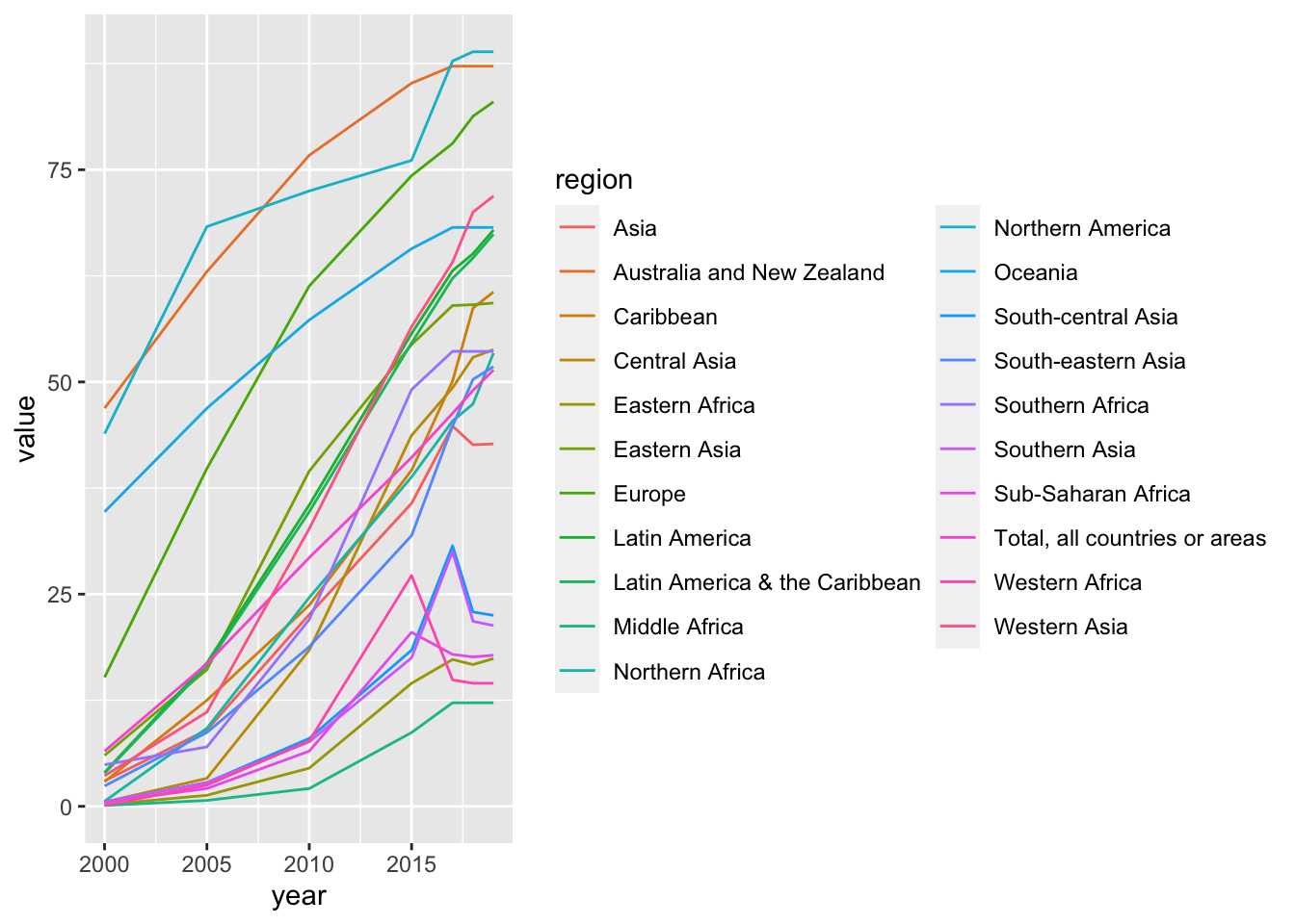

df_internet %>% filter(!(region %in% area_vector)) %>%
  ggplot(aes(x = factor(year), y = value)) + geom_boxplot() +
  labs(title = 'Percentage of individuals using the internet', x = 'year', y = 'percentage')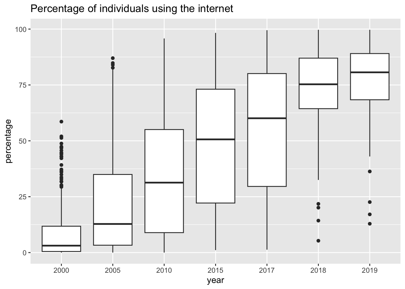

df_internet %>% filter(!(region %in% area_vector)) %>% filter(year %in% c(2000, 2005, 2010, 2015, 2019)) %>%
  ggplot(aes(x = value, color = factor(year))) + geom_freqpoly() +
  labs(title = 'Percentage of individuals using the internet', x = 'percentage')

## `stat_bin()` using `bins = 30`. Pick better value with `binwidth`.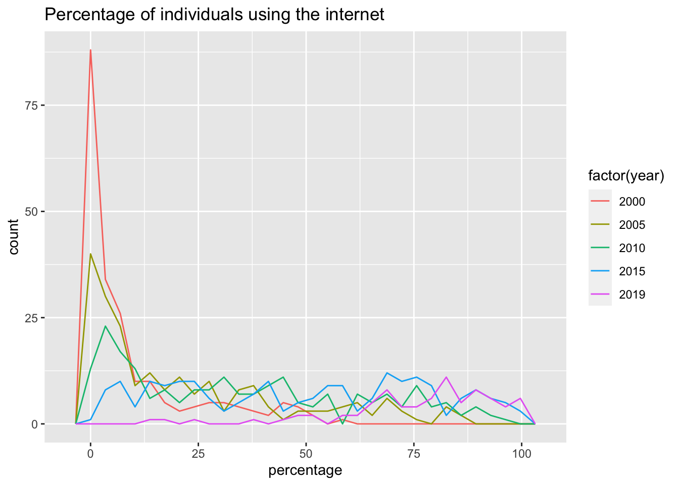

df_internet %>% filter(!(region %in% area_vector)) %>% filter(year == 2019) %>%
  ggplot(aes(x = value)) + geom_histogram() +
  labs(title = 'Percentage of individuals using the internet', x = 'percentage')

## `stat_bin()` using `bins = 30`. Pick better value with `binwidth`.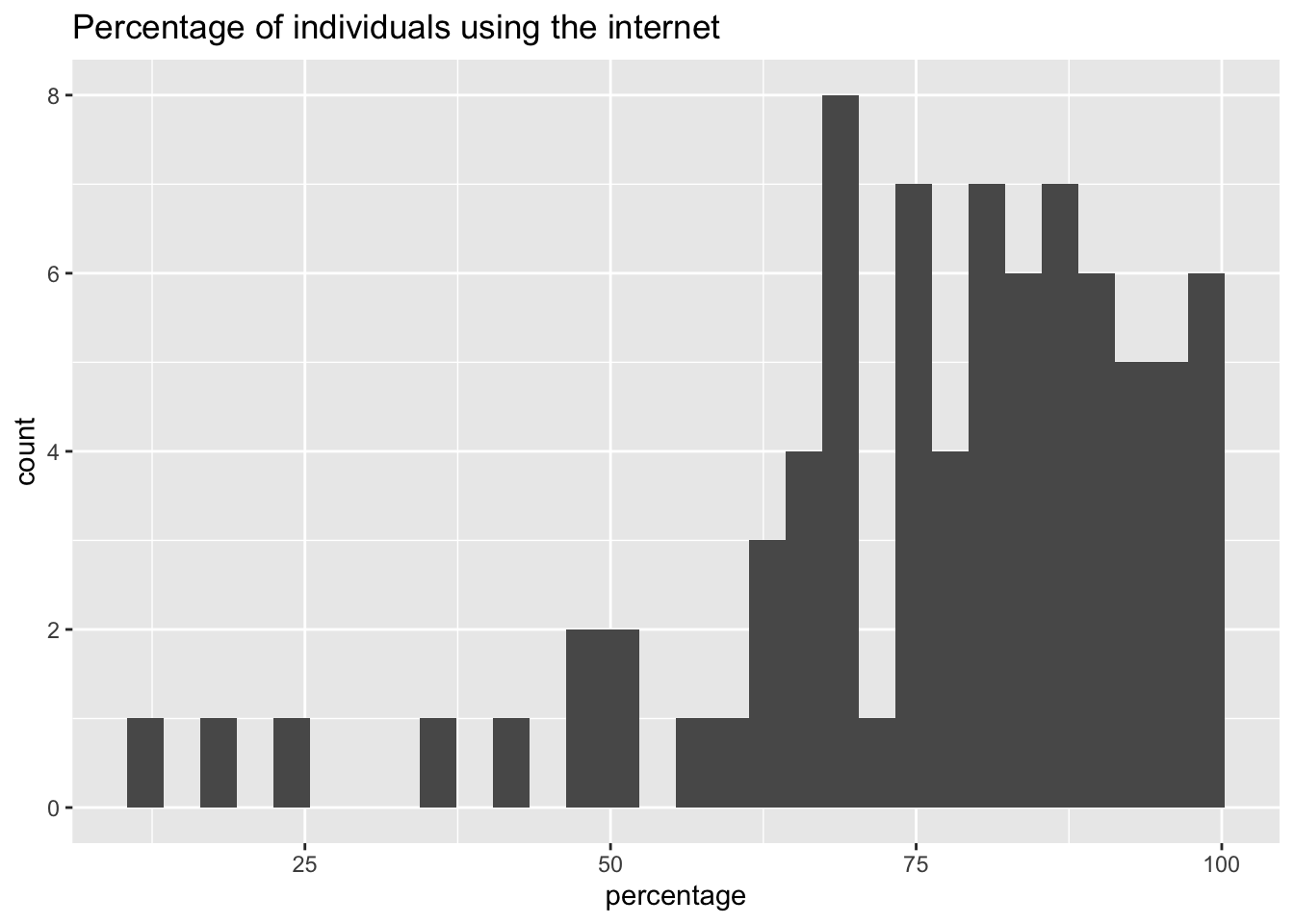

Only countries not in area_vector are used.
Medians are increasing.
There are lot of upper outliers in 2000 and 2005, and lower outliers in 2018 and 2020.

6.3.7.5 Modeling

df_internet %>% filter(region == "Total, all countries or areas") %>%
  ggplot(aes(x = year, y = value)) + geom_point() + geom_smooth(method = "lm", se = FALSE)

## `geom_smooth()` using formula = 'y ~ x'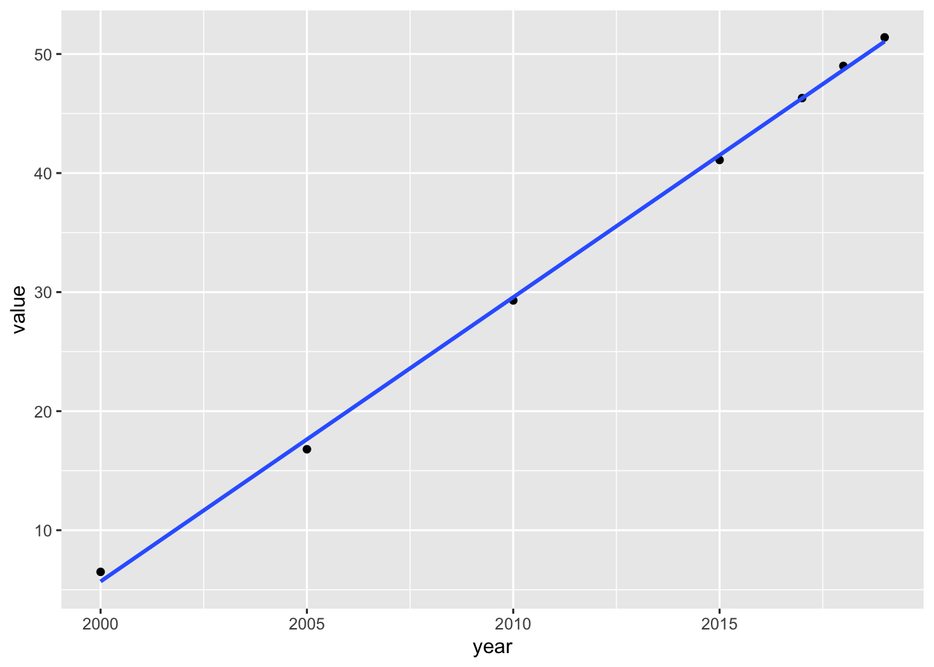

internet_all <- df_internet %>% filter(region == "Total, all countries or areas") %>%
  lm(value ~ year, .) 
internet_all %>%  summary()

## 
## Call:
## lm(formula = value ~ year, data = .)
## 
## Residuals:
##        1        2        3        4        5        6        7 
##  0.80524 -0.83146 -0.26817 -0.40488  0.02043  0.33309  0.34575 
## 
## Coefficients:
##               Estimate Std. Error t value Pr(>|t|)    
## (Intercept) -4.769e+03  6.803e+01   -70.1 1.12e-08 ***
## year         2.387e+00  3.381e-02    70.6 1.08e-08 ***
## ---
## Signif. codes:  0 '***' 0.001 '**' 0.01 '*' 0.05 '.' 0.1 ' ' 1
## 
## Residual standard error: 0.6011 on 5 degrees of freedom
## Multiple R-squared:  0.999,  Adjusted R-squared:  0.9988 
## F-statistic:  4985 on 1 and 5 DF,  p-value: 1.08e-08

Each year internet use is increasing by about 2.4 percents.

df_internet %>% filter(num %in% area_num_tmp) %>%
  ggplot(aes(x = year, y = value)) + geom_point() +
  geom_smooth(method = "lm", se = FALSE)

## `geom_smooth()` using formula = 'y ~ x'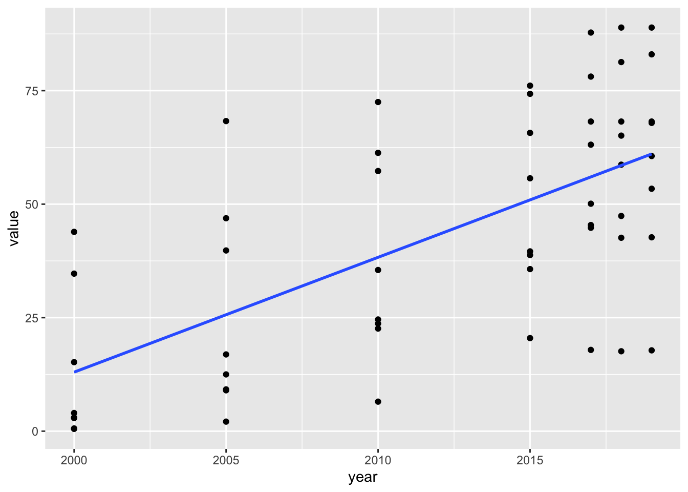

internet_area <- df_internet %>% filter(num %in% area_num_tmp) %>%
  lm(value ~ year, .)
internet_area  %>% summary()

## 
## Call:
## lm(formula = value ~ year, data = .)
## 
## Residuals:
##     Min      1Q  Median      3Q     Max 
## -43.255 -13.282  -4.344  19.570  42.655 
## 
## Coefficients:
##               Estimate Std. Error t value Pr(>|t|)    
## (Intercept) -5045.5456   827.6849  -6.096 1.20e-07 ***
## year            2.5293     0.4114   6.148 9.85e-08 ***
## ---
## Signif. codes:  0 '***' 0.001 '**' 0.01 '*' 0.05 '.' 0.1 ' ' 1
## 
## Residual standard error: 20.68 on 54 degrees of freedom
## Multiple R-squared:  0.4118, Adjusted R-squared:  0.4009 
## F-statistic:  37.8 on 1 and 54 DF,  p-value: 9.851e-08

df_internet %>% filter(!(region %in% area_vector)) %>%
  ggplot(aes(x = year, y = value)) + geom_point() +
  geom_smooth(method = "lm", se = FALSE)

## `geom_smooth()` using formula = 'y ~ x'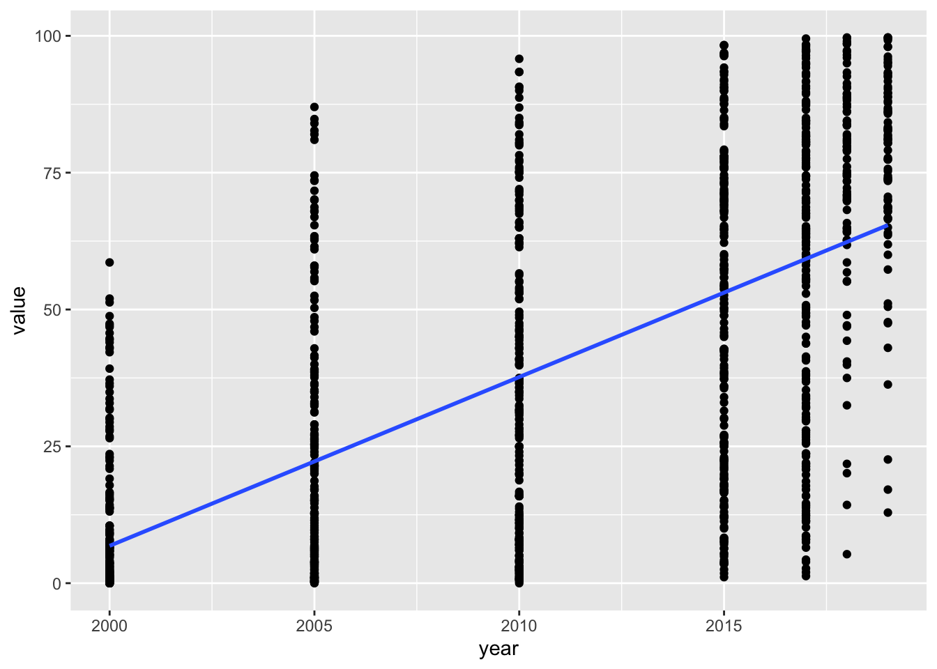

internet_country <- df_internet %>% filter(!(region %in% area_vector)) %>%
  lm(value ~ year, .) 
internet_country %>% summary()

## 
## Call:
## lm(formula = value ~ year, data = .)
## 
## Residuals:
##     Min      1Q  Median      3Q     Max 
## -57.950 -18.042  -1.026  18.268  64.755 
## 
## Coefficients:
##               Estimate Std. Error t value Pr(>|t|)    
## (Intercept) -6160.7035   214.9829  -28.66   <2e-16 ***
## year            3.0838     0.1069   28.84   <2e-16 ***
## ---
## Signif. codes:  0 '***' 0.001 '**' 0.01 '*' 0.05 '.' 0.1 ' ' 1
## 
## Residual standard error: 24.65 on 1208 degrees of freedom
## Multiple R-squared:  0.4078, Adjusted R-squared:  0.4073 
## F-statistic: 831.8 on 1 and 1208 DF,  p-value: < 2.2e-16

internet_summary <- list(ALL = internet_all, By_Area = internet_area, By_Country = internet_country)
msummary(internet_summary, statistic = 'p.value')

	ALL	By_Area	By_Country
(Intercept)	-4768.989	-5045.546	-6160.704
	(<0.001)	(<0.001)	(<0.001)
year	2.387	2.529	3.084
	(<0.001)	(<0.001)	(<0.001)
Num.Obs.	7	56	1210
R2	0.999	0.412	0.408
R2 Adj.	0.999	0.401	0.407
AIC	16.4	502.2	11193.3
BIC	16.2	508.2	11208.5
Log.Lik.	-5.192	-248.085	-5593.626
RMSE	0.51	20.31	24.63

What can you see? What are the difference of these three models? Which one is what you wanted? All aggreagated growth, growth by area, or growth by country of the internet use?

6.3.8 Bond Yields

6.3.8.1 Importing

Bonds and debentures are long-term securities that give the holders the unconditional right to one or both of: (a) a fixed or contractually determined variable money income in the form of coupon payments, i.e. payment of interest is not dependent on earnings of the debtors, (b) a stated fixed sum as a repayment of principal on a specified date or dates when the security is redeemed.
Data at United Nations: https://data.un.org/Data.aspx?q=bond+yeild&d=IFS&f=SeriesCode%3a61.
- Reach the site by search string “bond yields”
- Downloaded Data file in CSV: UNdata_Export_20220205_134850951.csv

df_by <- read_csv("data/UNdata_Export_20220205_134850951.csv")

## Rows: 2462 Columns: 6
## ── Column specification ──────────────────────────────────────────────────────────────────────────────────────────────────────
## Delimiter: ","
## chr (4): OID, Country or Area, Description, Magnitude
## dbl (2): Year, Value
## 
## ℹ Use `spec()` to retrieve the full column specification for this data.
## ℹ Specify the column types or set `show_col_types = FALSE` to quiet this message.

6.3.8.2 Glimpsing

df_by

## # A tibble: 2,462 × 6
##    OID           `Country or Area`  Year Description              Magnit…¹ Value
##    <chr>         <chr>             <dbl> <chr>                    <chr>    <dbl>
##  1 91161...ZF... ARMENIA            2007 GOVERNMENT BOND YIELD    PERCENT…  6.56
##  2 91161...ZF... ARMENIA            2006 GOVERNMENT BOND YIELD    PERCENT…  5.86
##  3 91161...ZF... ARMENIA            2005 GOVERNMENT BOND YIELD    PERCENT…  5.18
##  4 91161...ZF... ARMENIA            2004 GOVERNMENT BOND YIELD    PERCENT…  8.21
##  5 91161...ZF... ARMENIA            2003 GOVERNMENT BOND YIELD    PERCENT… 15.7 
##  6 91161...ZF... ARMENIA            2002 GOVERNMENT BOND YIELD    PERCENT… 17.4 
##  7 91161...ZF... ARMENIA            2001 GOVERNMENT BOND YIELD    PERCENT… 23.2 
##  8 91161...ZF... ARMENIA            2000 GOVERNMENT BOND YIELD    PERCENT… 25.5 
##  9 19361A..ZF... AUSTRALIA          2009 TREASURY BONDS: 3 YEARS  PERCENT…  4.26
## 10 19361...ZF... AUSTRALIA          2009 TREASURY BONDS: 15 YEARS PERCENT…  5.09
## # … with 2,452 more rows, and abbreviated variable name ¹Magnitude

df_by %>% glimpse()

## Rows: 2,462
## Columns: 6
## $ OID               <chr> "91161...ZF...", "91161...ZF...", "91161...ZF...", "…
## $ `Country or Area` <chr> "ARMENIA", "ARMENIA", "ARMENIA", "ARMENIA", "ARMENIA…
## $ Year              <dbl> 2007, 2006, 2005, 2004, 2003, 2002, 2001, 2000, 2009…
## $ Description       <chr> "GOVERNMENT BOND YIELD", "GOVERNMENT BOND YIELD", "G…
## $ Magnitude         <chr> "PERCENT PER ANNU", "PERCENT PER ANNU", "PERCENT PER…
## $ Value             <dbl> 6.56222, 5.85693, 5.18325, 8.20862, 15.71420, 17.442…

df_by %>% distinct(Description)

## # A tibble: 33 × 1
##    Description                    
##    <chr>                          
##  1 GOVERNMENT BOND YIELD          
##  2 TREASURY BONDS: 3 YEARS        
##  3 TREASURY BONDS: 15 YEARS       
##  4 GOV. BONDS: 10 YEARS           
##  5 GOVERNMENT BOND YEILD          
##  6 GOVT BOND YIELD 3-5 YEARS      
##  7 GOVERNMENT BOND YIELD > 10 YRS.
##  8 GOVT. BOND YIELD               
##  9 MORTGAGE BOND YIELD            
## 10 LONG-TERM LOAN RATE            
## # … with 23 more rows

df_by %>% group_by(Description) %>% summarize(num_of_regions = n_distinct(`Country or Area`)) %>%
  arrange(desc(num_of_regions))

## # A tibble: 33 × 2
##    Description                          num_of_regions
##    <chr>                                         <int>
##  1 GOVERNMENT BOND YIELD                            44
##  2 15 YEAR TREASURY BOND YIELD                       1
##  3 5 YEAR TREASURY BOND YIELD                        1
##  4 AVG SHT TRM GOVT BONDS RATE                       1
##  5 COUPON RATE ON L.T.DEVELPT BONDS                  1
##  6 GOV. BONDS: 10 YEARS                              1
##  7 GOVENMENT BOND YIELD                              1
##  8 GOVERNMENT BOND RATE                              1
##  9 GOVERNMENT BOND YEILD                             1
## 10 GOVERNMENT BOND YIELD - 10 YEAR IND.              1
## # … with 23 more rows

df_by %>% filter(Description == "GOVERNMENT BOND YIELD") %>%
  distinct(OID, `Country or Area`, Description)

## # A tibble: 44 × 3
##    OID           `Country or Area` Description          
##    <chr>         <chr>             <chr>                
##  1 91161...ZF... ARMENIA           GOVERNMENT BOND YIELD
##  2 12261...ZF... AUSTRIA           GOVERNMENT BOND YIELD
##  3 12461...ZF... BELGIUM           GOVERNMENT BOND YIELD
##  4 93561...ZF... CZECH REPUBLIC    GOVERNMENT BOND YIELD
##  5 12861...ZF... DENMARK           GOVERNMENT BOND YIELD
##  6 64461...ZF... ETHIOPIA          GOVERNMENT BOND YIELD
##  7 16361...ZF... EURO AREA         GOVERNMENT BOND YIELD
##  8 17261...ZF... FINLAND           GOVERNMENT BOND YIELD
##  9 13261...ZF... FRANCE            GOVERNMENT BOND YIELD
## 10 13461...ZF... GERMANY           GOVERNMENT BOND YIELD
## # … with 34 more rows

df_by %>% filter(Description != "GOVERNMENT BOND YIELD") %>%
  distinct(OID, `Country or Area`, Description)

## # A tibble: 32 × 3
##    OID           `Country or Area` Description                    
##    <chr>         <chr>             <chr>                          
##  1 19361A..ZF... AUSTRALIA         TREASURY BONDS: 3 YEARS        
##  2 19361...ZF... AUSTRALIA         TREASURY BONDS: 15 YEARS       
##  3 61661...ZF... BOTSWANA          GOV. BONDS: 10 YEARS           
##  4 91861...ZF... BULGARIA          GOVERNMENT BOND YEILD          
##  5 15661A..ZF... CANADA            GOVT BOND YIELD 3-5 YEARS      
##  6 15661...ZF... CANADA            GOVERNMENT BOND YIELD > 10 YRS.
##  7 42361...ZF... CYPRUS            GOVT. BOND YIELD               
##  8 12861A..ZF... DENMARK           MORTGAGE BOND YIELD            
##  9 93961...ZF... ESTONIA           LONG-TERM LOAN RATE            
## 10 81961...ZF... FIJI              AVG SHT TRM GOVT BONDS RATE    
## # … with 22 more rows

df_by %>% distinct(Magnitude)

## # A tibble: 1 × 1
##   Magnitude       
##   <chr>           
## 1 PERCENT PER ANNU

df_by %>% distinct(Year) %>% arrange(desc(Year))

## # A tibble: 62 × 1
##     Year
##    <dbl>
##  1  2009
##  2  2008
##  3  2007
##  4  2006
##  5  2005
##  6  2004
##  7  2003
##  8  2002
##  9  2001
## 10  2000
## # … with 52 more rows

df_by %>% group_by(Year) %>% summarize(number_of_countries = n_distinct(`Country or Area`)) %>%
  arrange(desc(number_of_countries))

## # A tibble: 62 × 2
##     Year number_of_countries
##    <dbl>               <int>
##  1  2006                  61
##  2  2005                  60
##  3  2007                  59
##  4  2004                  58
##  5  2003                  57
##  6  2002                  54
##  7  2001                  53
##  8  2008                  53
##  9  1995                  47
## 10  2000                  47
## # … with 52 more rows

df_by %>% distinct(OID)

## # A tibble: 76 × 1
##    OID          
##    <chr>        
##  1 91161...ZF...
##  2 19361A..ZF...
##  3 19361...ZF...
##  4 12261...ZF...
##  5 12461...ZF...
##  6 61661...ZF...
##  7 91861...ZF...
##  8 15661A..ZF...
##  9 15661...ZF...
## 10 42361...ZF...
## # … with 66 more rows

df_by %>% distinct(`Country or Area`)

## # A tibble: 69 × 1
##    `Country or Area`
##    <chr>            
##  1 ARMENIA          
##  2 AUSTRALIA        
##  3 AUSTRIA          
##  4 BELGIUM          
##  5 BOTSWANA         
##  6 BULGARIA         
##  7 CANADA           
##  8 CYPRUS           
##  9 CZECH REPUBLIC   
## 10 DENMARK          
## # … with 59 more rows

df_by %>% distinct(OID, `Country or Area`)

## # A tibble: 76 × 2
##    OID           `Country or Area`
##    <chr>         <chr>            
##  1 91161...ZF... ARMENIA          
##  2 19361A..ZF... AUSTRALIA        
##  3 19361...ZF... AUSTRALIA        
##  4 12261...ZF... AUSTRIA          
##  5 12461...ZF... BELGIUM          
##  6 61661...ZF... BOTSWANA         
##  7 91861...ZF... BULGARIA         
##  8 15661A..ZF... CANADA           
##  9 15661...ZF... CANADA           
## 10 42361...ZF... CYPRUS           
## # … with 66 more rows

df_by %>% group_by(`Country or Area`) %>% summarize(num_of_oid = n_distinct(OID)) %>%
  arrange(desc(num_of_oid))

## # A tibble: 69 × 2
##    `Country or Area` num_of_oid
##    <chr>                  <int>
##  1 AUSTRALIA                  2
##  2 CANADA                     2
##  3 DENMARK                    2
##  4 ITALY                      2
##  5 MOROCCO                    2
##  6 UNITED KINGDOM             2
##  7 UNITED STATES              2
##  8 ARMENIA                    1
##  9 AUSTRIA                    1
## 10 BELGIUM                    1
## # … with 59 more rows

Seven countries have two OID and others have one OID.

6.3.8.3 Visualising

df_by %>% filter(`Country or Area` == 'JAPAN') %>%
  ggplot(aes(x = Year, y = Value)) +
  geom_line()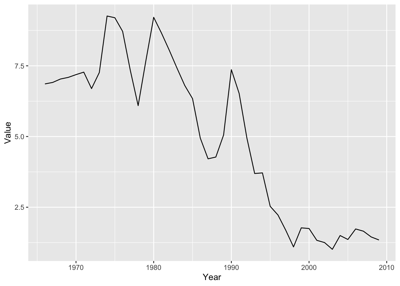

df_by %>% filter(`Country or Area` %in% c('FRANCE', 'GERMANY', 'GREECE', 'CHINA', 'INDIA', 'JAPAN', 'PAKISTAN')) %>%
  ggplot(aes(x = Year, y = Value, color = `Country or Area`)) +
  geom_line()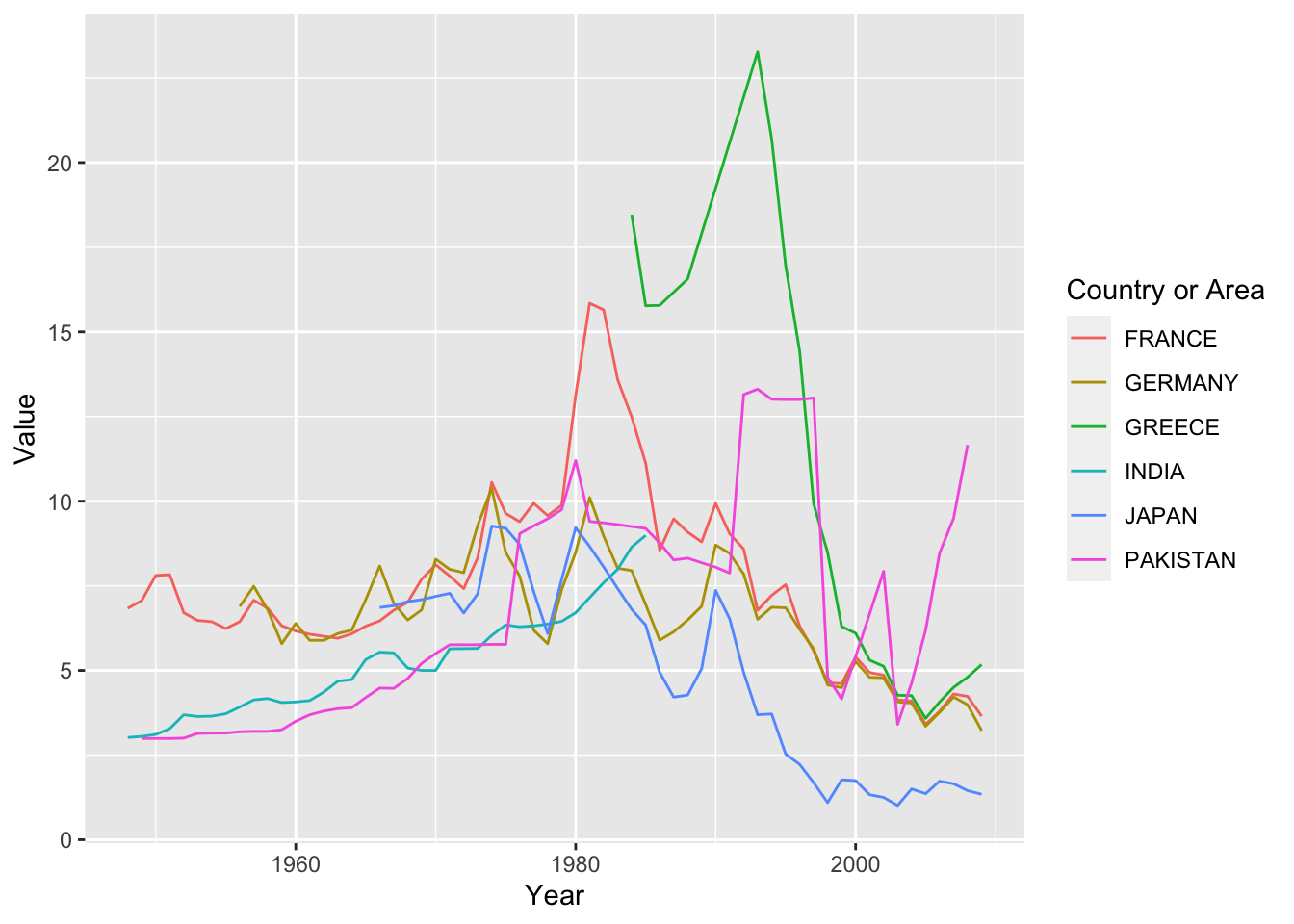

6.3.8.4 Modeling

df_by %>% filter(`Country or Area` %in% c('JAPAN')) %>%
  ggplot(aes(x = Year, y = Value)) +
  geom_line() +
    geom_smooth(method = "lm", se = FALSE)

## `geom_smooth()` using formula = 'y ~ x'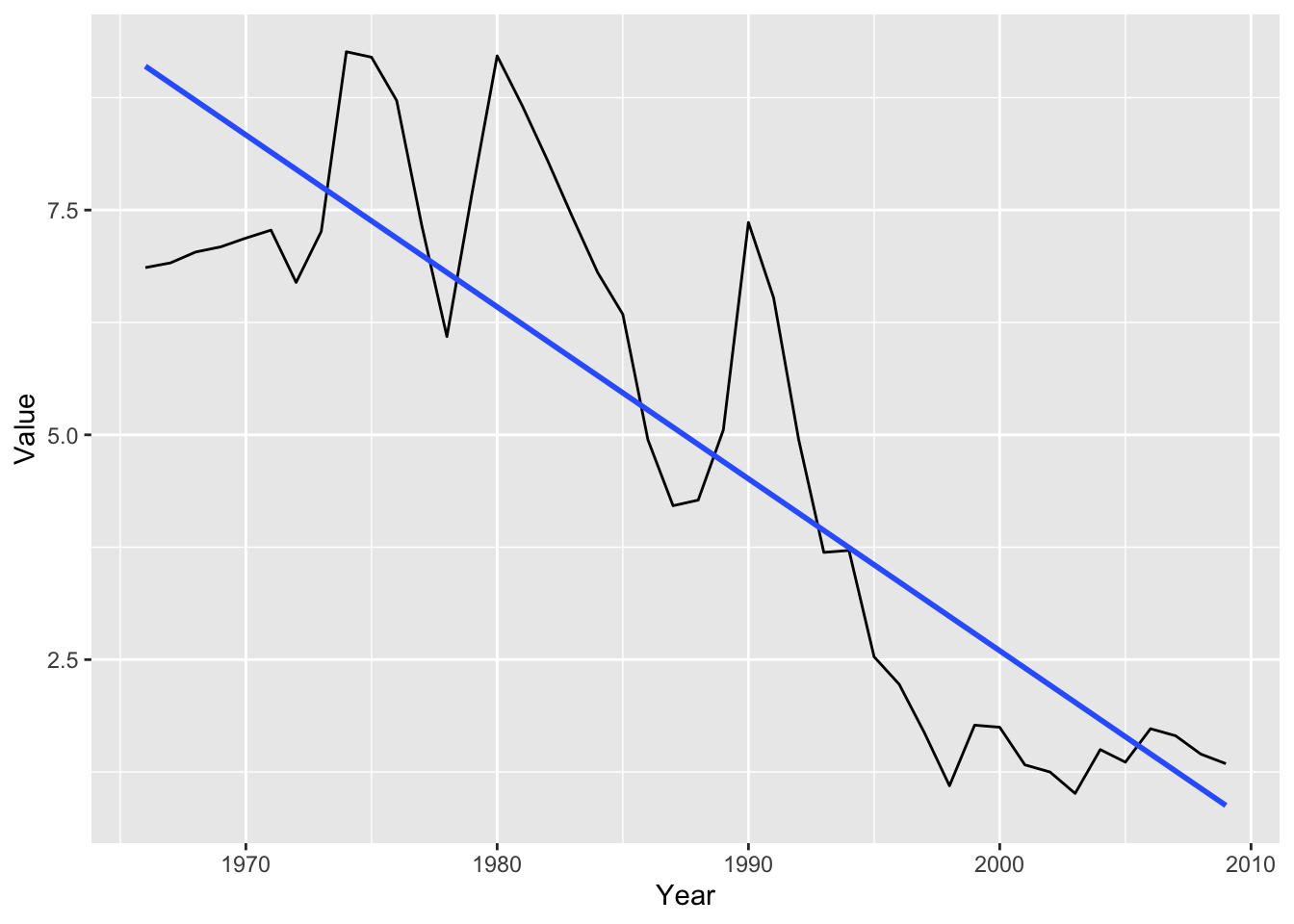

df_by %>% filter(`Country or Area` %in% c('JAPAN')) %>%
  lm(Value ~ Year, .) %>% summary()

## 
## Call:
## lm(formula = Value ~ Year, data = .)
## 
## Residuals:
##     Min      1Q  Median      3Q     Max 
## -2.2402 -1.0199 -0.3071  0.9237  2.8517 
## 
## Coefficients:
##              Estimate Std. Error t value Pr(>|t|)    
## (Intercept) 385.05294   32.41293   11.88 5.15e-15 ***
## Year         -0.19123    0.01631  -11.73 7.86e-15 ***
## ---
## Signif. codes:  0 '***' 0.001 '**' 0.01 '*' 0.05 '.' 0.1 ' ' 1
## 
## Residual standard error: 1.374 on 42 degrees of freedom
## Multiple R-squared:  0.766,  Adjusted R-squared:  0.7604 
## F-statistic: 137.5 on 1 and 42 DF,  p-value: 7.864e-15

df_by %>% filter(Description %in% c('GOVERNMENT BOND YIELD')) %>%
  ggplot(aes(x = Year, y = Value)) +
  scale_y_log10() +
  geom_point() + geom_smooth(method = "lm")

## `geom_smooth()` using formula = 'y ~ x'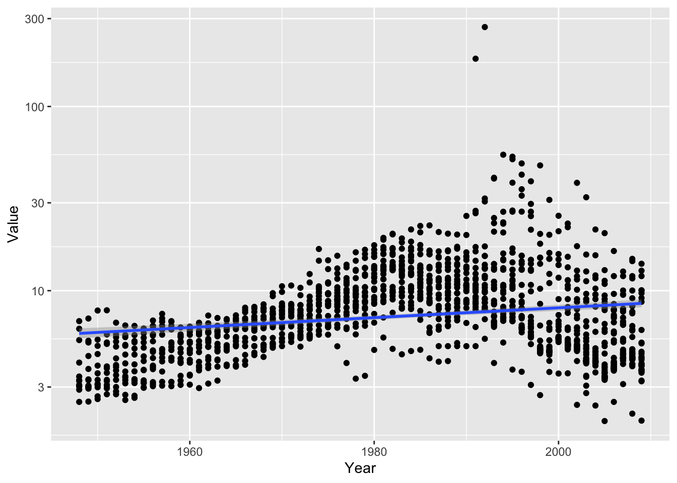

df_by %>% filter(Description %in% c('GOVERNMENT BOND YIELD')) %>% filter(Year >=1980) %>% 
  ggplot(aes(x = Year, y = Value)) +
  scale_y_log10() +
  geom_point() + geom_smooth(method = "lm")

## `geom_smooth()` using formula = 'y ~ x'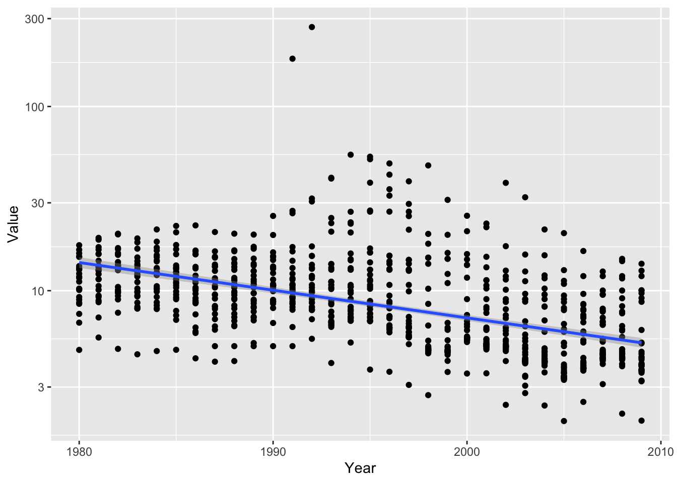

df_by %>% filter(Description %in% c('GOVERNMENT BOND YIELD')) %>% filter(Year >=1980) %>% 
  lm(Value ~ Year, .) %>% summary()

## 
## Call:
## lm(formula = Value ~ Year, data = .)
## 
## Residuals:
##     Min      1Q  Median      3Q     Max 
## -10.041  -3.619  -2.251   0.882 258.725 
## 
## Coefficients:
##              Estimate Std. Error t value Pr(>|t|)    
## (Intercept) 599.57505   93.60857   6.405 2.43e-10 ***
## Year         -0.29534    0.04691  -6.296 4.79e-10 ***
## ---
## Signif. codes:  0 '***' 0.001 '**' 0.01 '*' 0.05 '.' 0.1 ' ' 1
## 
## Residual standard error: 12.07 on 888 degrees of freedom
## Multiple R-squared:  0.04273,    Adjusted R-squared:  0.04165 
## F-statistic: 39.64 on 1 and 888 DF,  p-value: 4.793e-10

Very small R squared value, however we can see a downward trend as the coefficient of Year is about -0.3.

6.3.9 Elderly Population

6.3.9.1 Importing

OECD website: https://data.oecd.org/
- Choose from “topic”, “Society”, and then “Elderly population”
  - URL: https://data.oecd.org/pop/elderly-population.htm
- We can copy the URL of the download data
The elderly population is defined as people aged 65 and over.

Use of CLASS.xls

url_oecd_elderly <- "https://stats.oecd.org/sdmx-json/data/DP_LIVE/.ELDLYPOP.TOT.PC_POP.A/OECD?contentType=csv&detail=code&separator=comma&csv-lang=en&startPeriod=1970"

elderly_population <- read_csv(url_oecd_elderly)

## Rows: 2909 Columns: 8
## ── Column specification ──────────────────────────────────────────────────────────────────────────────────────────────────────
## Delimiter: ","
## chr (5): LOCATION, INDICATOR, SUBJECT, MEASURE, FREQUENCY
## dbl (2): TIME, Value
## lgl (1): Flag Codes
## 
## ℹ Use `spec()` to retrieve the full column specification for this data.
## ℹ Specify the column types or set `show_col_types = FALSE` to quiet this message.

6.3.9.2 Glimpsing

elderly_population

## # A tibble: 2,909 × 8
##    LOCATION INDICATOR SUBJECT MEASURE FREQUENCY  TIME Value `Flag Codes`
##    <chr>    <chr>     <chr>   <chr>   <chr>     <dbl> <dbl> <lgl>       
##  1 AUS      ELDLYPOP  TOT     PC_POP  A          1970  8.35 NA          
##  2 AUS      ELDLYPOP  TOT     PC_POP  A          1971  8.34 NA          
##  3 AUS      ELDLYPOP  TOT     PC_POP  A          1972  8.41 NA          
##  4 AUS      ELDLYPOP  TOT     PC_POP  A          1973  8.51 NA          
##  5 AUS      ELDLYPOP  TOT     PC_POP  A          1974  8.61 NA          
##  6 AUS      ELDLYPOP  TOT     PC_POP  A          1975  8.72 NA          
##  7 AUS      ELDLYPOP  TOT     PC_POP  A          1976  8.93 NA          
##  8 AUS      ELDLYPOP  TOT     PC_POP  A          1977  9.07 NA          
##  9 AUS      ELDLYPOP  TOT     PC_POP  A          1978  9.24 NA          
## 10 AUS      ELDLYPOP  TOT     PC_POP  A          1979  9.44 NA          
## # … with 2,899 more rows

elderly_population %>% distinct(INDICATOR)

## # A tibble: 1 × 1
##   INDICATOR
##   <chr>    
## 1 ELDLYPOP

elderly_population %>% distinct(SUBJECT)

## # A tibble: 1 × 1
##   SUBJECT
##   <chr>  
## 1 TOT

elderly_population %>% distinct(MEASURE)

## # A tibble: 1 × 1
##   MEASURE
##   <chr>  
## 1 PC_POP

elderly_population %>% distinct(FREQUENCY)

## # A tibble: 1 × 1
##   FREQUENCY
##   <chr>    
## 1 A

elderly_population %>% distinct(`Flag Codes`)

## # A tibble: 1 × 1
##   `Flag Codes`
##   <lgl>       
## 1 NA

6.3.9.3 Transforming

elderly_pop <- elderly_population %>% select(iso3c = LOCATION, year = TIME, value = Value)

elderly_pop

## # A tibble: 2,909 × 3
##    iso3c  year value
##    <chr> <dbl> <dbl>
##  1 AUS    1970  8.35
##  2 AUS    1971  8.34
##  3 AUS    1972  8.41
##  4 AUS    1973  8.51
##  5 AUS    1974  8.61
##  6 AUS    1975  8.72
##  7 AUS    1976  8.93
##  8 AUS    1977  9.07
##  9 AUS    1978  9.24
## 10 AUS    1979  9.44
## # … with 2,899 more rows

elderly_pop_ext <- elderly_pop %>% left_join(wb_countries, by = 'iso3c') 
elderly_pop_ext

## # A tibble: 2,909 × 8
##    iso3c  year value country   region              income      lending other
##    <chr> <dbl> <dbl> <chr>     <chr>               <chr>       <chr>   <chr>
##  1 AUS    1970  8.35 Australia East Asia & Pacific High income <NA>    <NA> 
##  2 AUS    1971  8.34 Australia East Asia & Pacific High income <NA>    <NA> 
##  3 AUS    1972  8.41 Australia East Asia & Pacific High income <NA>    <NA> 
##  4 AUS    1973  8.51 Australia East Asia & Pacific High income <NA>    <NA> 
##  5 AUS    1974  8.61 Australia East Asia & Pacific High income <NA>    <NA> 
##  6 AUS    1975  8.72 Australia East Asia & Pacific High income <NA>    <NA> 
##  7 AUS    1976  8.93 Australia East Asia & Pacific High income <NA>    <NA> 
##  8 AUS    1977  9.07 Australia East Asia & Pacific High income <NA>    <NA> 
##  9 AUS    1978  9.24 Australia East Asia & Pacific High income <NA>    <NA> 
## 10 AUS    1979  9.44 Australia East Asia & Pacific High income <NA>    <NA> 
## # … with 2,899 more rows

elderly_pop_ext %>% distinct(iso3c, country)

## # A tibble: 56 × 2
##    iso3c country       
##    <chr> <chr>         
##  1 AUS   Australia     
##  2 AUT   Austria       
##  3 BEL   Belgium       
##  4 CAN   Canada        
##  5 CZE   Czech Republic
##  6 DNK   Denmark       
##  7 FIN   Finland       
##  8 FRA   France        
##  9 DEU   Germany       
## 10 GRC   Greece        
## # … with 46 more rows

6.3.9.4 Visualising

The following render the same chart.

elderly_pop_ext %>% filter(year == 2020, !is.na(region)) %>%
  ggplot(aes(region, fill = income)) + geom_bar() + coord_flip()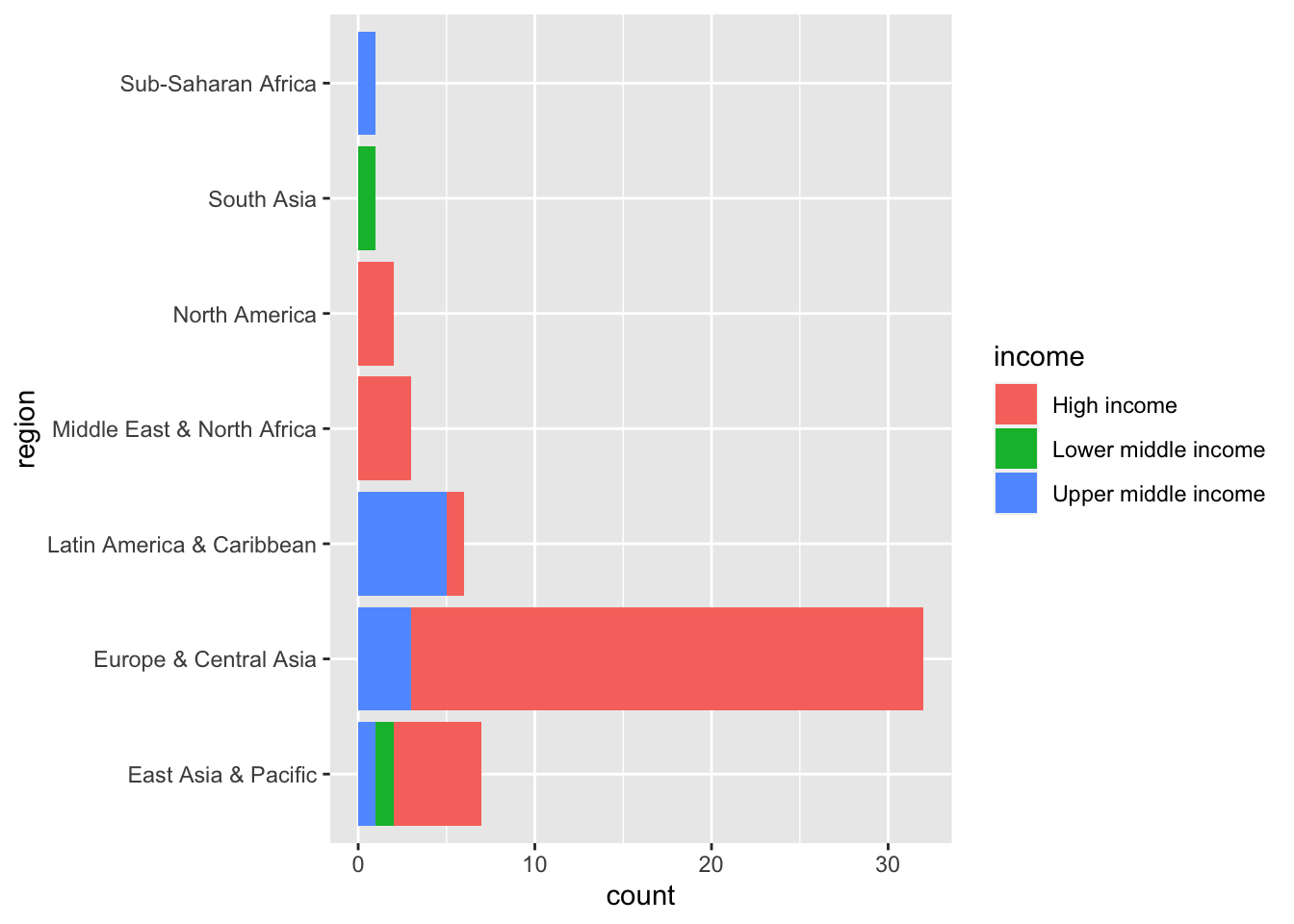

elderly_pop_ext %>% filter(year == 2020, !is.na(region)) %>%
  ggplot(aes(y = region, fill = income)) + geom_bar(orientation = "y")

elderly_pop_ext %>% filter(iso3c %in% c("AUS", "CAN", "DEU", "FRA", "GBR", "JPN", "KOR", "USA")) %>%
  ggplot(aes(x = year, y = value, color = country)) +
  geom_line()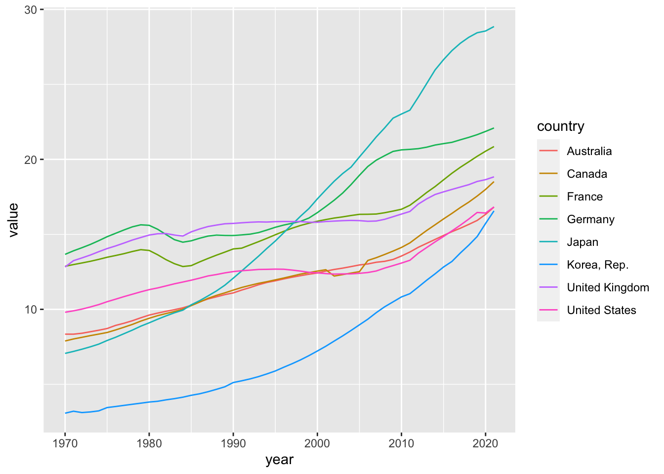

elderly_pop_ext %>% filter(income == "High income") %>%
  ggplot(aes(x = year, y = value, color = country)) +
  geom_line() + 
  labs(title = "High income")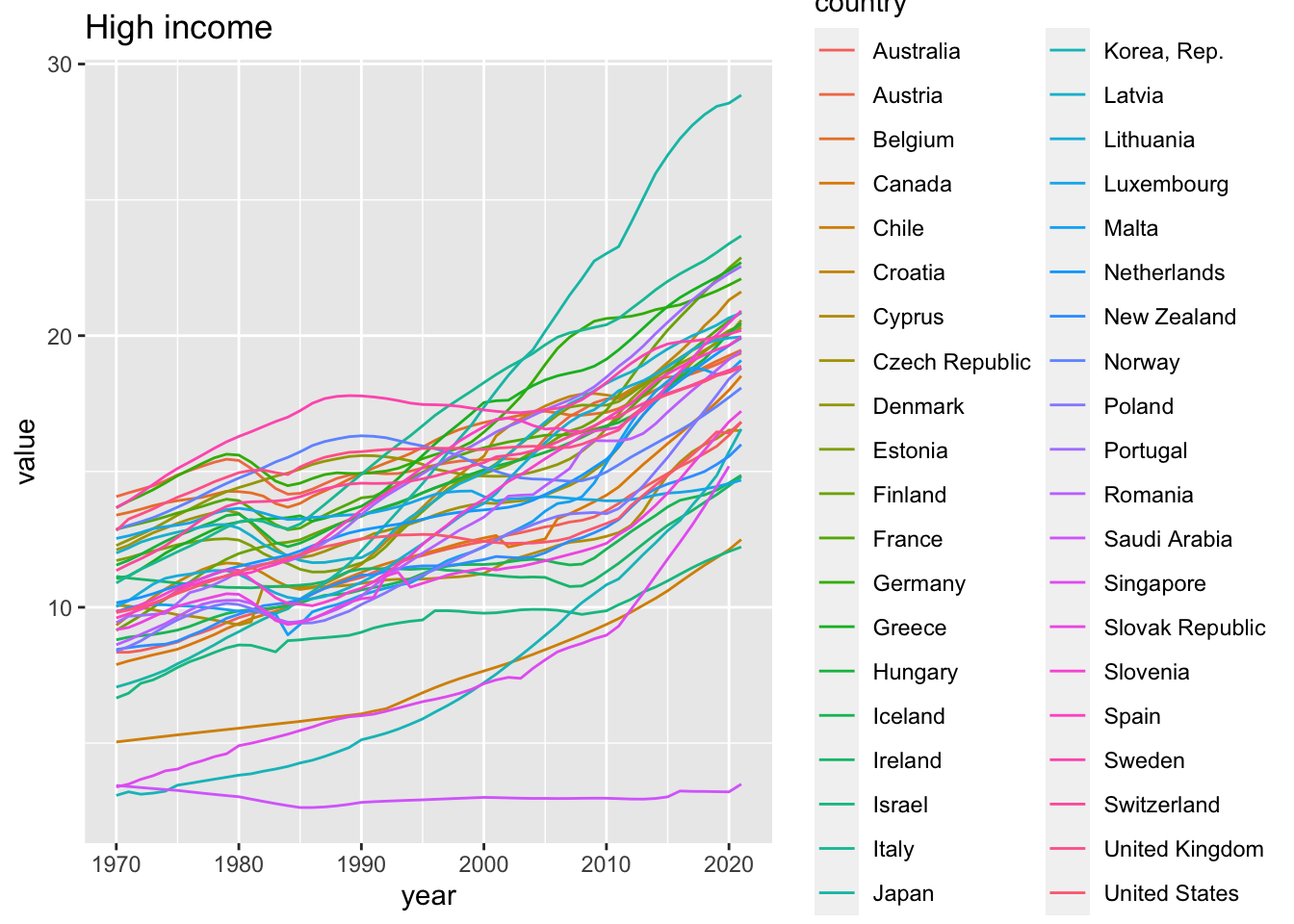

elderly_pop_ext %>% filter(income == "Upper middle income") %>%
  ggplot(aes(x = year, y = value, color = country)) +
  geom_line() + 
  labs(title = "Upper middle income")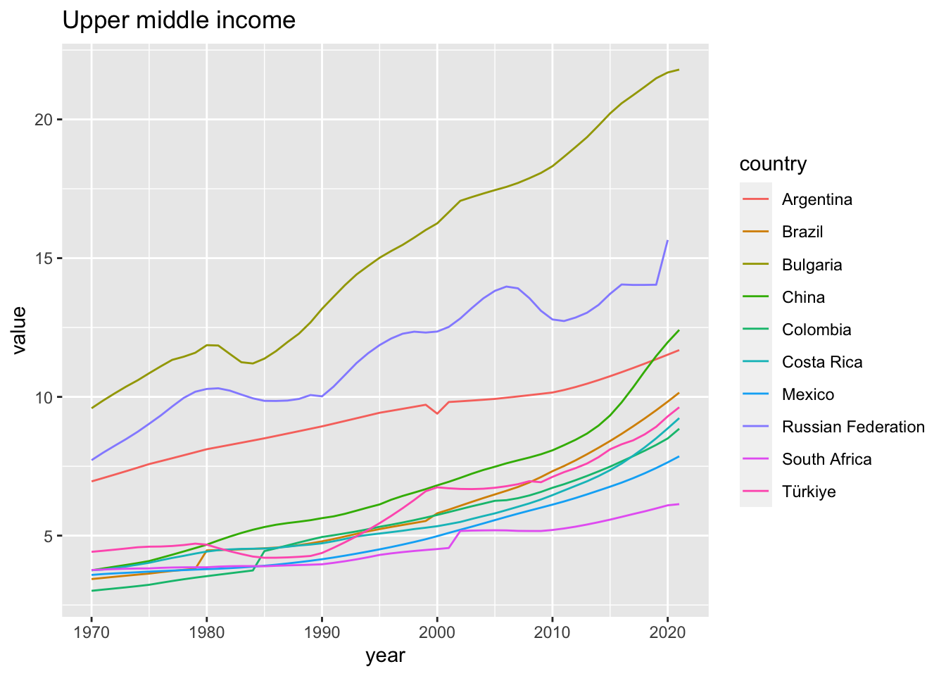

elderly_pop_ext %>% filter(income == "Lower middle income") %>%
  ggplot(aes(x = year, y = value, color = country)) +
  geom_line() + 
  labs(title = "Lower middle income")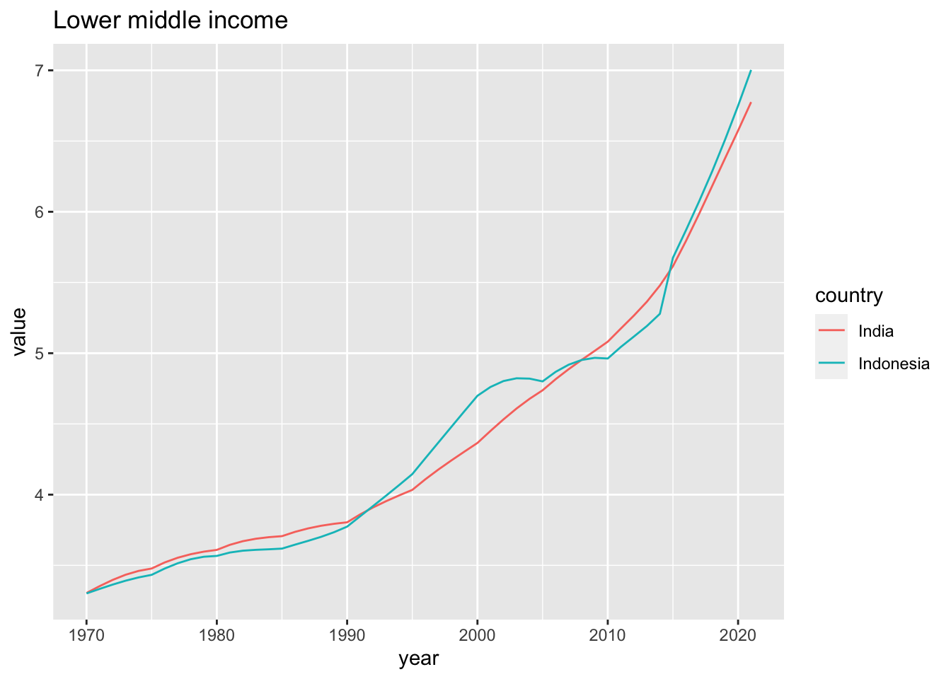

#### Modeling

elderly_pop_all <- elderly_pop_ext %>% 
  lm(value ~ year, .)
elderly_pop_all %>% summary()

## 
## Call:
## lm(formula = value ~ year, data = .)
## 
## Residuals:
##      Min       1Q   Median       3Q      Max 
## -12.0913  -3.6968   0.7292   3.3638  13.4150 
## 
## Coefficients:
##               Estimate Std. Error t value Pr(>|t|)    
## (Intercept) -275.96633   10.49675  -26.29   <2e-16 ***
## year           0.14419    0.00526   27.41   <2e-16 ***
## ---
## Signif. codes:  0 '***' 0.001 '**' 0.01 '*' 0.05 '.' 0.1 ' ' 1
## 
## Residual standard error: 4.254 on 2907 degrees of freedom
## Multiple R-squared:  0.2054, Adjusted R-squared:  0.2051 
## F-statistic: 751.4 on 1 and 2907 DF,  p-value: < 2.2e-16

elderly_pop_high <- elderly_pop_ext %>% filter(income == "High income") %>%
  lm(value ~ year, .)
elderly_pop_high %>% summary()

## 
## Call:
## lm(formula = value ~ year, data = .)
## 
## Residuals:
##      Min       1Q   Median       3Q      Max 
## -13.9763  -1.6256   0.4638   2.2517  11.5163 
## 
## Coefficients:
##               Estimate Std. Error t value Pr(>|t|)    
## (Intercept) -3.018e+02  9.756e+00  -30.93   <2e-16 ***
## year         1.579e-01  4.889e-03   32.30   <2e-16 ***
## ---
## Signif. codes:  0 '***' 0.001 '**' 0.01 '*' 0.05 '.' 0.1 ' ' 1
## 
## Residual standard error: 3.344 on 2077 degrees of freedom
## Multiple R-squared:  0.3344, Adjusted R-squared:  0.334 
## F-statistic:  1043 on 1 and 2077 DF,  p-value: < 2.2e-16

elderly_pop_upper_middle <- elderly_pop_ext %>% filter(income == "Upper middle income") %>%
  lm(value ~ year, .)
elderly_pop_upper_middle %>% summary()

## 
## Call:
## lm(formula = value ~ year, data = .)
## 
## Residuals:
##    Min     1Q Median     3Q    Max 
## -4.198 -2.219 -1.372  1.987 11.470 
## 
## Coefficients:
##               Estimate Std. Error t value Pr(>|t|)    
## (Intercept) -2.161e+02  1.991e+01  -10.85   <2e-16 ***
## year         1.120e-01  9.977e-03   11.23   <2e-16 ***
## ---
## Signif. codes:  0 '***' 0.001 '**' 0.01 '*' 0.05 '.' 0.1 ' ' 1
## 
## Residual standard error: 3.405 on 517 degrees of freedom
## Multiple R-squared:  0.196,  Adjusted R-squared:  0.1945 
## F-statistic: 126.1 on 1 and 517 DF,  p-value: < 2.2e-16

elderly_pop_lower_middle <- elderly_pop_ext %>% filter(income == "Lower middle income") %>%
  lm(value ~ year, .)
elderly_pop_lower_middle %>% summary()

## 
## Call:
## lm(formula = value ~ year, data = .)
## 
## Residuals:
##      Min       1Q   Median       3Q      Max 
## -0.35190 -0.24233 -0.09253  0.20393  1.07837 
## 
## Coefficients:
##               Estimate Std. Error t value Pr(>|t|)    
## (Intercept) -1.137e+02  4.039e+00  -28.16   <2e-16 ***
## year         5.920e-02  2.024e-03   29.25   <2e-16 ***
## ---
## Signif. codes:  0 '***' 0.001 '**' 0.01 '*' 0.05 '.' 0.1 ' ' 1
## 
## Residual standard error: 0.3097 on 102 degrees of freedom
## Multiple R-squared:  0.8935, Adjusted R-squared:  0.8924 
## F-statistic: 855.6 on 1 and 102 DF,  p-value: < 2.2e-16

elderly_pop_summary <- list(ALL = elderly_pop_all,High = elderly_pop_high, Upper_middle = elderly_pop_upper_middle, Loer_middle = elderly_pop_lower_middle)
msummary(elderly_pop_summary, statistic = 'p.value')

	ALL	High	Upper_middle	Loer_middle
(Intercept)	-275.966	-301.813	-216.065	-113.712
	(<0.001)	(<0.001)	(<0.001)	(<0.001)
year	0.144	0.158	0.112	0.059
	(<0.001)	(<0.001)	(<0.001)	(<0.001)
Num.Obs.	2909	2079	519	104
R2	0.205	0.334	0.196	0.893
R2 Adj.	0.205	0.334	0.194	0.892
AIC	16682.8	10923.6	2748.7	55.3
BIC	16700.7	10940.5	2761.4	63.3
Log.Lik.	-8338.381	-5458.809	-1371.326	-24.672
RMSE	4.25	3.34	3.40	0.31

All data show the increase of the population of elderly people.
There are differences in income level. Can you sess? Look at year, the slope.
Can we state that they are significangly different? It is a statistical problem.

6.3.10 Education

6.3.10.1 Importing

Go to UN data website: https://data.un.org/
At the bottom in popular statistical tables, scroll to education
download from “education at the primary, secondary and tertiary level”

edu_tmp <- read_csv("data/edu.csv", skip = 1, n_max =6942) %>% slice(-1)

## New names:
## Rows: 6940 Columns: 7
## ── Column specification
## ──────────────────────────────────────────────────────────────────────────────────────────────────────
## Delimiter: "," chr (4): ...2, Series, Footnotes, Source dbl (2): Region/Country/Area, Year num (1): Value
## ℹ Use `spec()` to retrieve the full column specification for this data. ℹ Specify the column types or set `show_col_types =
## FALSE` to quiet this message.
## • `` -> `...2`

edu_tmp

## # A tibble: 6,939 × 7
##    `Region/Country/Area` ...2                  Year Series  Value Footn…¹ Source
##                    <dbl> <chr>                <dbl> <chr>   <dbl> <chr>   <chr> 
##  1                     1 Total, all countrie…  2005 Gross… 1.04e2 <NA>    Unite…
##  2                     1 Total, all countrie…  2005 Gross… 9.97e1 <NA>    Unite…
##  3                     1 Total, all countrie…  2005 Stude… 5.09e5 <NA>    Unite…
##  4                     1 Total, all countrie…  2005 Gross… 6.58e1 <NA>    Unite…
##  5                     1 Total, all countrie…  2005 Gross… 6.23e1 <NA>    Unite…
##  6                     1 Total, all countrie…  2005 Stude… 2.00e5 <NA>    Unite…
##  7                     1 Total, all countrie…  2005 Gross… 5.12e1 <NA>    Unite…
##  8                     1 Total, all countrie…  2005 Gross… 4.83e1 <NA>    Unite…
##  9                     1 Total, all countrie…  2010 Stude… 6.97e5 <NA>    Unite…
## 10                     1 Total, all countrie…  2010 Gross… 1.04e2 <NA>    Unite…
## # … with 6,929 more rows, and abbreviated variable name ¹Footnotes

6.3.10.2 Transforming

edu_data <- edu_tmp %>% select(`Region/Country/Area`:Source)
edu_data

## # A tibble: 6,939 × 7
##    `Region/Country/Area` ...2                  Year Series  Value Footn…¹ Source
##                    <dbl> <chr>                <dbl> <chr>   <dbl> <chr>   <chr> 
##  1                     1 Total, all countrie…  2005 Gross… 1.04e2 <NA>    Unite…
##  2                     1 Total, all countrie…  2005 Gross… 9.97e1 <NA>    Unite…
##  3                     1 Total, all countrie…  2005 Stude… 5.09e5 <NA>    Unite…
##  4                     1 Total, all countrie…  2005 Gross… 6.58e1 <NA>    Unite…
##  5                     1 Total, all countrie…  2005 Gross… 6.23e1 <NA>    Unite…
##  6                     1 Total, all countrie…  2005 Stude… 2.00e5 <NA>    Unite…
##  7                     1 Total, all countrie…  2005 Gross… 5.12e1 <NA>    Unite…
##  8                     1 Total, all countrie…  2005 Gross… 4.83e1 <NA>    Unite…
##  9                     1 Total, all countrie…  2010 Stude… 6.97e5 <NA>    Unite…
## 10                     1 Total, all countrie…  2010 Gross… 1.04e2 <NA>    Unite…
## # … with 6,929 more rows, and abbreviated variable name ¹Footnotes

colnames(edu_data)

## [1] "Region/Country/Area" "...2"                "Year"               
## [4] "Series"              "Value"               "Footnotes"          
## [7] "Source"

edu_tidy <- edu_data %>%
  select(country = `...2`, year = Year, series = Series, value = Value)
edu_tidy

## # A tibble: 6,939 × 4
##    country                        year series                              value
##    <chr>                         <dbl> <chr>                               <dbl>
##  1 Total, all countries or areas  2005 Gross enrollment ratio - Primary … 1.04e2
##  2 Total, all countries or areas  2005 Gross enrollment ratio - Primary … 9.97e1
##  3 Total, all countries or areas  2005 Students enrolled in secondary ed… 5.09e5
##  4 Total, all countries or areas  2005 Gross enrollment ratio - Secondar… 6.58e1
##  5 Total, all countries or areas  2005 Gross enrollment ratio - Secondar… 6.23e1
##  6 Total, all countries or areas  2005 Students enrolled in upper second… 2.00e5
##  7 Total, all countries or areas  2005 Gross enrollment ratio - Upper se… 5.12e1
##  8 Total, all countries or areas  2005 Gross enrollment ratio - Upper se… 4.83e1
##  9 Total, all countries or areas  2010 Students enrolled in primary educ… 6.97e5
## 10 Total, all countries or areas  2010 Gross enrollment ratio - Primary … 1.04e2
## # … with 6,929 more rows

edu_tidy %>% distinct(series)

## # A tibble: 9 × 1
##   series                                                    
##   <chr>                                                     
## 1 Gross enrollment ratio - Primary (male)                   
## 2 Gross enrollment ratio - Primary (female)                 
## 3 Students enrolled in secondary education (thousands)      
## 4 Gross enrollment ratio - Secondary (male)                 
## 5 Gross enrollment ratio - Secondary (female)               
## 6 Students enrolled in upper secondary education (thousands)
## 7 Gross enrollment ratio - Upper secondary level (male)     
## 8 Gross enrollment ratio - Upper secondary level (female)   
## 9 Students enrolled in primary education (thousands)

edu_tidy %>% group_by(year) %>% summarize(n = n_distinct(country)) %>% arrange(desc(n))

## # A tibble: 15 × 2
##     year     n
##    <dbl> <int>
##  1  2005   198
##  2  2015   187
##  3  2010   186
##  4  2019   106
##  5  2018    78
##  6  2009    25
##  7  2014    16
##  8  2017    16
##  9  2016    15
## 10  2007    11
## 11  2008    11
## 12  2012    11
## 13  2013    10
## 14  2006     7
## 15  2011     6

6.3.10.3 Modeling

From the correlation, we can see R squared values.

edu_tidy %>% filter(year == 2019) %>% 
  pivot_wider(names_from = series, values_from = value) %>% select(primary = 3, secondary = 6, tertiary = 9) %>% drop_na %>% 
  cor()

##             primary secondary  tertiary
## primary   1.0000000 0.9968584 0.9927488
## secondary 0.9968584 1.0000000 0.9987411
## tertiary  0.9927488 0.9987411 1.0000000

edu_tidy %>% filter(year == 2019) %>% 
  pivot_wider(names_from = series, values_from = value) %>% select(primary = 3, p_male = 4, p_female = 5, secondary = 6, s_mele = 7, s_female = 8, tertiary = 9, t_male = 10, t_female = 11) %>% drop_na %>% 
  cor()

##               primary      p_male    p_female   secondary      s_mele
## primary    1.00000000 -0.04596002 -0.06210728  0.99681390 -0.05181750
## p_male    -0.04596002  1.00000000  0.91721150 -0.05414662  0.06900585
## p_female  -0.06210728  0.91721150  1.00000000 -0.06803863  0.15039583
## secondary  0.99681390 -0.05414662 -0.06803863  1.00000000 -0.03978368
## s_mele    -0.05181750  0.06900585  0.15039583 -0.03978368  1.00000000
## s_female  -0.05582660  0.06878992  0.16237304 -0.04326115  0.97846907
## tertiary   0.99263244 -0.05881375 -0.07088605  0.99872764 -0.04128023
## t_male    -0.03978945 -0.07399155 -0.01141148 -0.02545667  0.86547359
## t_female  -0.05676420 -0.04125532  0.01764835 -0.04271911  0.88976428
##              s_female    tertiary      t_male    t_female
## primary   -0.05582660  0.99263244 -0.03978945 -0.05676420
## p_male     0.06878992 -0.05881375 -0.07399155 -0.04125532
## p_female   0.16237304 -0.07088605 -0.01141148  0.01764835
## secondary -0.04326115  0.99872764 -0.02545667 -0.04271911
## s_mele     0.97846907 -0.04128023  0.86547359  0.88976428
## s_female   1.00000000 -0.04502461  0.85201284  0.91859578
## tertiary  -0.04502461  1.00000000 -0.02458739 -0.04279010
## t_male     0.85201284 -0.02458739  1.00000000  0.95488259
## t_female   0.91859578 -0.04279010  0.95488259  1.00000000

edu_tidy %>% filter(year == 2019) %>% 
  pivot_wider(names_from = series, values_from = value) %>% 
  select(primary = 3, secondary = 6, tertiary = 9) %>% 
  drop_na %>%
  ggplot(aes(x = secondary, y = tertiary)) + geom_point() + geom_smooth(method = "lm", se = FALSE)

## `geom_smooth()` using formula = 'y ~ x'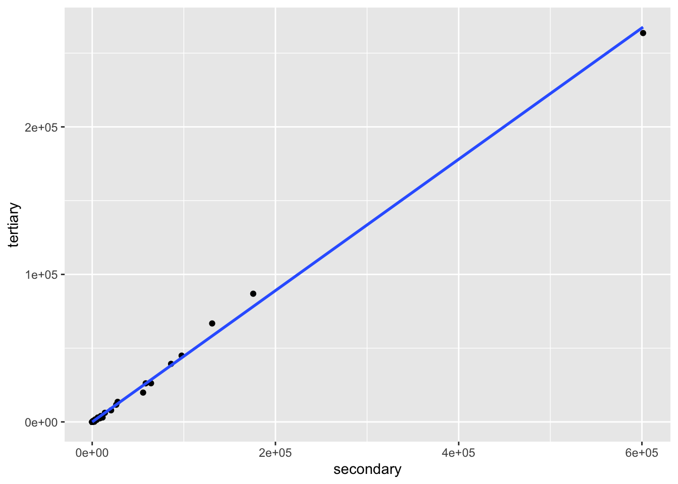

edu_tidy %>% filter(year == 2019) %>% 
  pivot_wider(names_from = series, values_from = value) %>% 
  select(primary = 3, secondary = 6, tertiary = 9) %>% 
  drop_na %>%
  filter(secondary < 100000) %>% 
  ggplot(aes(x = secondary, y = tertiary)) + geom_point() + geom_smooth(method = "lm", se = FALSE)

## `geom_smooth()` using formula = 'y ~ x'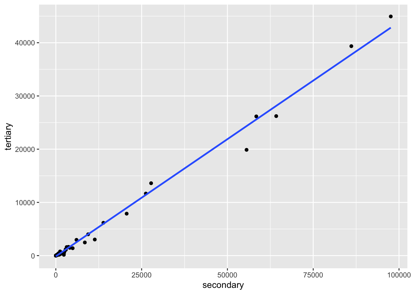

edu_tidy %>% filter(year == 2019) %>% 
  pivot_wider(names_from = series, values_from = value) %>% 
  select(primary = 3, secondary = 6, tertiary = 9) %>% 
  drop_na %>%
  lm(tertiary ~ secondary, .) %>% summary()

## 
## Call:
## lm(formula = tertiary ~ secondary, data = .)
## 
## Residuals:
##     Min      1Q  Median      3Q     Max 
## -4857.3  -130.4    -2.2     5.6  8678.4 
## 
## Coefficients:
##               Estimate Std. Error t value Pr(>|t|)    
## (Intercept)  -3.185597 172.385304  -0.018    0.985    
## secondary     0.445145   0.002425 183.568   <2e-16 ***
## ---
## Signif. codes:  0 '***' 0.001 '**' 0.01 '*' 0.05 '.' 0.1 ' ' 1
## 
## Residual standard error: 1563 on 85 degrees of freedom
## Multiple R-squared:  0.9975, Adjusted R-squared:  0.9975 
## F-statistic: 3.37e+04 on 1 and 85 DF,  p-value: < 2.2e-16