E Appendix E Population

Population Analysis using the UN Data and the US Census Bureau

E.1 About: United States Census Bureau

The Unites States of America Census Burea compiles a huge set of data. It provides data to the World Fact Book of Central Intelligence Agency and the Census Academy resources for Data Science Education.

In alignment with the Digital Government Strategy, the Census Bureau is offering the public wider access to key U.S. statistics. (About)

To study the population analysis of the world and its visualization, visit the following sites:

Census Academy: https://www.census.gov/data/academy.html
Infographics & Visualizations: https://www.census.gov/library/visualizations.html
U.S. and World Population Clock: https://www.census.gov/popclock/world
Data Tool: https://www.census.gov/data-tools/demo/idb/#/country?YR_ANIM=2020

We can access to the data directly or by an API, Application Program Interface. In the following we study population data of the world in these two ways.

E.2 International Data Base (IDB) December 2020 Release (Now in 2021)

These data files correspond to the data available in the U.S. Census Bureau’s API. Each file is pipe “|” delimited, and the header row is demarcated with “#” at the start of the row. For additional technical specifications, including variable definitions, please visit https://www.census.gov/data/developers/data-sets/international-database.html

For more information about the International Data Base, including release notes and detailed methodology, please visit https://www.census.gov/programs-surveys/international-programs/about/idb.html

Variables:
- AGE: Single year of age from 0-100+
- AREA_KM2: Area in square kilometers
- FIPS: FIPS country/area Code Federal Information Processing Standards
- for: Census API FIPS ‘for’ clause
- GENC: Geopolitical Entities, Names, and Codes (GENC) two character country code standard
- in: Census API FIPS ‘in’ clause
- NAME Country or area name
- POP: Total mid-year population
- SEX: Sex 0 = Both Sexes, 1 = Male, 2 = Female
- time: ISO-8601 Date/Time value
- ucgid Uniform Census Geography Identifier clause
- YR Year

The file size is huge as a text file with about 8 million rows. (For Excel, the total number of rows on a worksheet is 1,048,576, about 1 million.) We need to download once but we should read the downloaded file instead of downloading it everytime. Commands in tidyverse package works very fast and we can handle the data of this size.

Recently 2021 version was publishes: https://www.census.gov/data-tools/demo/idb/#/country?YR_ANIM=2021
New: https://www2.census.gov/programs-surveys/international-programs/about/idb/idbzip.zip
Old: https://www2.census.gov/programs-surveys/international-programs/about/idb/idbzip.zip

E.3 Analysis using `idbzip`

library(tidyverse)

### For the first time, delete # in the following four lines to download the files.
## From the second time, add # to the following four lines to avoid downloading the files.
# idbzip_url <- "https://www2.census.gov/programs-surveys/international-programs/about/idb/idbzip.zip" # URL of the zip file.
# dir.create("data/idbzip") # store everything in idbzip directory in the working directory
# download.file(url = idbzip_url, destfile = "data/idbzip/idbzip.zip") # file size: 43.1 MB
# unzip("data/idbzip/idbzip.zip", exdir = "data/idbzip") # zip file contains three files idb5yr.all, idbsingleyear.all, Readme.txt

# idb <- read_delim("data/idbzip/idbsingleyear.all", delim = "|")
# glimpse(idb)
# idb

Since it is too large, we chose 15 countries and stored it as data/idb15.csv and data/world.csv, which is the data of the world population.

#idb %>% 
#  filter(GENC %in% c("BD", "CH","DE","FR","GB","ID", "IN","JP", "KR","LK","MY", "PH","TH","US","VN"))  %>%
#  select("YEAR" = `#YR`, "COUNTRY" = NAME, "ISO2" = GENC, SEX, POP, AGE) %>%
#  write_csv("data/idb15.csv")

world_all <- idb %>% 
  select("YEAR" = `#YR`, SEX, POP, AGE) %>%
  mutate(SEX = as_factor(SEX))
world <- world_all %>% 
  group_by(YEAR, SEX) %>%
  summarize(POPULATION = sum(POP))
world
write_csv(world, "data/world.csv")

countries <- idb %>% 
  select("YEAR" = `#YR`, SEX, GENC, POP) %>%
  mutate(SEX = as_factor(SEX)) %>% filter(SEX == 0) %>%
  group_by(YEAR, GENC) %>%
  summarize(POPULATION = sum(POP)) %>%
  ungroup() %>%
  group_by(YEAR) %>% 
  summarize(NUMBER = n())
write_csv(countries, "data/world2.csv")

E.3.1 Popultion of the World

world <- read_csv("data/world.csv")

## Rows: 453 Columns: 3
## ── Column specification ──────────────────────────────────────────────────────────────────────────────────────────────────────
## Delimiter: ","
## dbl (3): YEAR, SEX, POPULATION
## 
## ℹ Use `spec()` to retrieve the full column specification for this data.
## ℹ Specify the column types or set `show_col_types = FALSE` to quiet this message.

world2 <- read_csv("data/world2.csv")

## Rows: 151 Columns: 2
## ── Column specification ──────────────────────────────────────────────────────────────────────────────────────────────────────
## Delimiter: ","
## dbl (2): YEAR, NUMBER
## 
## ℹ Use `spec()` to retrieve the full column specification for this data.
## ℹ Specify the column types or set `show_col_types = FALSE` to quiet this message.

idb15 <- read_csv("data/idb15.csv")

## Rows: 509343 Columns: 6
## ── Column specification ──────────────────────────────────────────────────────────────────────────────────────────────────────
## Delimiter: ","
## chr (2): COUNTRY, ISO2
## dbl (4): YEAR, SEX, POP, AGE
## 
## ℹ Use `spec()` to retrieve the full column specification for this data.
## ℹ Specify the column types or set `show_col_types = FALSE` to quiet this message.

idb15

## # A tibble: 509,343 × 6
##     YEAR COUNTRY    ISO2    SEX     POP   AGE
##    <dbl> <chr>      <chr> <dbl>   <dbl> <dbl>
##  1  1981 Bangladesh BD        0 3428071     0
##  2  1981 Bangladesh BD        0 3072594     1
##  3  1981 Bangladesh BD        0 2888362     2
##  4  1981 Bangladesh BD        0 2782738     3
##  5  1981 Bangladesh BD        0 2719081     4
##  6  1981 Bangladesh BD        0 2669809     5
##  7  1981 Bangladesh BD        0 2614671     6
##  8  1981 Bangladesh BD        0 2545849     7
##  9  1981 Bangladesh BD        0 2462867     8
## 10  1981 Bangladesh BD        0 2373595     9
## # … with 509,333 more rows

idb15 %>% distinct(COUNTRY, ISO2)

## # A tibble: 15 × 2
##    COUNTRY        ISO2 
##    <chr>          <chr>
##  1 Bangladesh     BD   
##  2 China          CN   
##  3 Germany        DE   
##  4 France         FR   
##  5 United Kingdom GB   
##  6 Indonesia      ID   
##  7 India          IN   
##  8 Japan          JP   
##  9 Korea, South   KR   
## 10 Sri Lanka      LK   
## 11 Malaysia       MY   
## 12 Philippines    PH   
## 13 Thailand       TH   
## 14 United States  US   
## 15 Vietnam        VN

summary(idb15)

##       YEAR        COUNTRY              ISO2                SEX   
##  Min.   :1980   Length:509343      Length:509343      Min.   :0  
##  1st Qu.:2014   Class :character   Class :character   1st Qu.:0  
##  Median :2042   Mode  :character   Mode  :character   Median :1  
##  Mean   :2042                                         Mean   :1  
##  3rd Qu.:2070                                         3rd Qu.:2  
##  Max.   :2100                                         Max.   :2  
##       POP                AGE     
##  Min.   :       6   Min.   :  0  
##  1st Qu.:  253533   1st Qu.: 25  
##  Median :  516669   Median : 50  
##  Mean   : 1813595   Mean   : 50  
##  3rd Qu.: 1329090   3rd Qu.: 75  
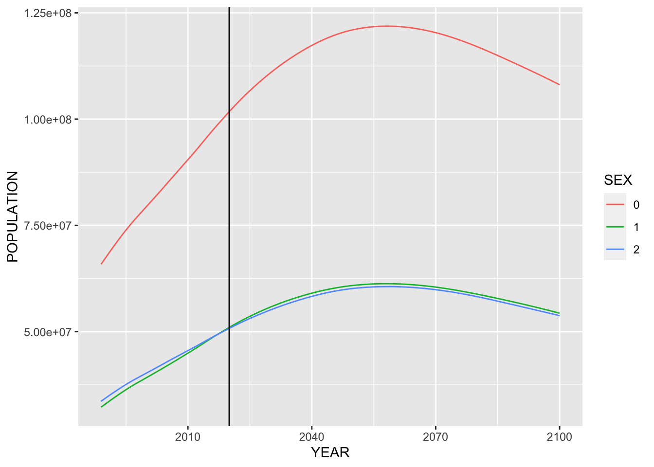
##  Max.   :30630618   Max.   :100

world %>% ggplot(aes(x = YEAR, y = POPULATION)) +
  geom_line(aes(color = SEX)) + 
  geom_vline(xintercept = 2020)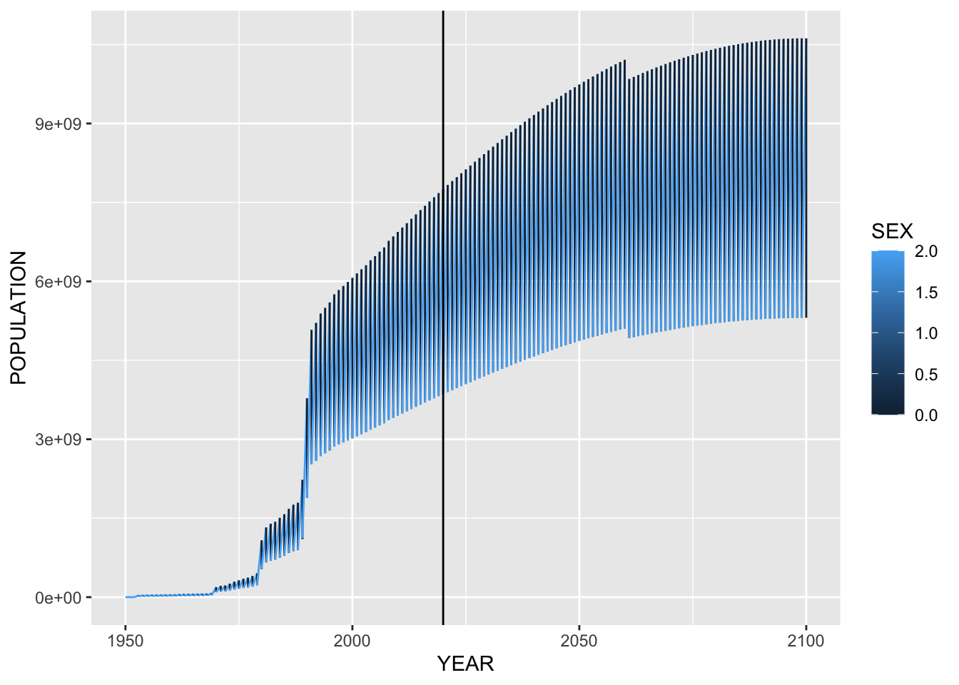

Something is wrong!

summary(world2)

##       YEAR          NUMBER     
##  Min.   :1950   Min.   :  2.0  
##  1st Qu.:1988   1st Qu.:113.5  
##  Median :2025   Median :226.0  
##  Mean   :2025   Mean   :173.3  
##  3rd Qu.:2062   3rd Qu.:227.0  
##  Max.   :2100   Max.   :227.0

ggplot(world2, aes(x = YEAR, y = NUMBER)) +
  geom_bar(stat = "identity")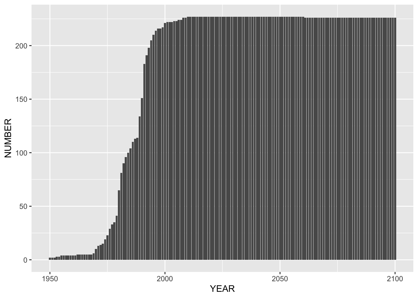

E.3.2 Population of a Country, JAPAN

japan <- filter(idb15, ISO2 == "JP") %>% select(YEAR, SEX, POP, AGE) %>%
  mutate(SEX = as_factor(SEX))
japan

## # A tibble: 33,633 × 4
##     YEAR SEX       POP   AGE
##    <dbl> <fct>   <dbl> <dbl>
##  1  1990 0     1228598     0
##  2  1990 0     1275792     1
##  3  1990 0     1318661     2
##  4  1990 0     1355679     3
##  5  1990 0     1388504     4
##  6  1990 0     1452576     5
##  7  1990 0     1494424     6
##  8  1990 0     1507634     7
##  9  1990 0     1515567     8
## 10  1990 0     1547527     9
## # … with 33,623 more rows

pop <- japan %>% group_by(YEAR, SEX) %>% summarize(POPULATION = sum(POP))

## `summarise()` has grouped output by 'YEAR'. You can override using the `.groups`
## argument.

pop

## # A tibble: 333 × 3
## # Groups:   YEAR [111]
##     YEAR SEX   POPULATION
##    <dbl> <fct>      <dbl>
##  1  1990 0      123537399
##  2  1990 1       60628417
##  3  1990 2       62908982
##  4  1991 0      123962538
##  5  1991 1       60832741
##  6  1991 2       63129797
##  7  1992 0      124378689
##  8  1992 1       61030495
##  9  1992 2       63348194
## 10  1993 0      124738157
## # … with 323 more rows

pop %>% ggplot(aes(x = YEAR, y = POPULATION)) +
  geom_line(aes(color = SEX)) + 
  geom_vline(xintercept = 2020)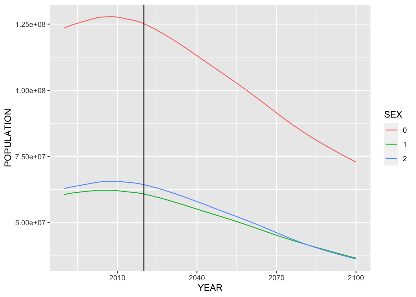

japan2020 <- japan %>% filter(YEAR == 2020, SEX == 0)
ggplot(japan2020) +
  geom_bar(aes(x = AGE, y = POP), stat = "identity")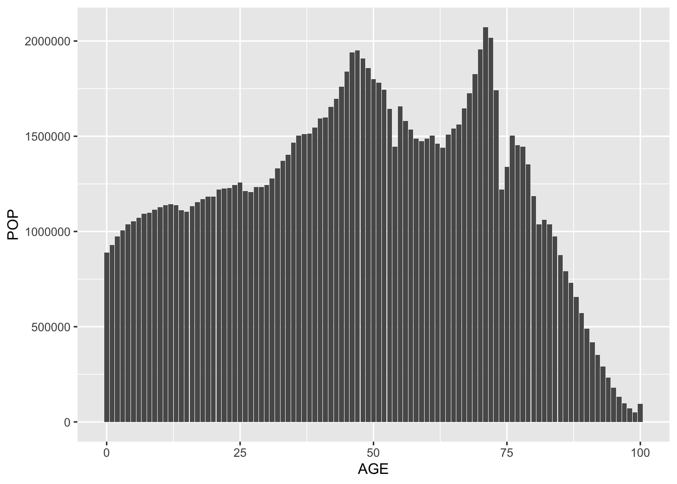

japan_adult <- filter(japan2020, AGE >=18) 
ggplot(japan_adult) +
  geom_line(aes(x = AGE, y = cumsum(POP)/sum(POP)*100)) + 
  geom_vline(xintercept = 40, color = "red")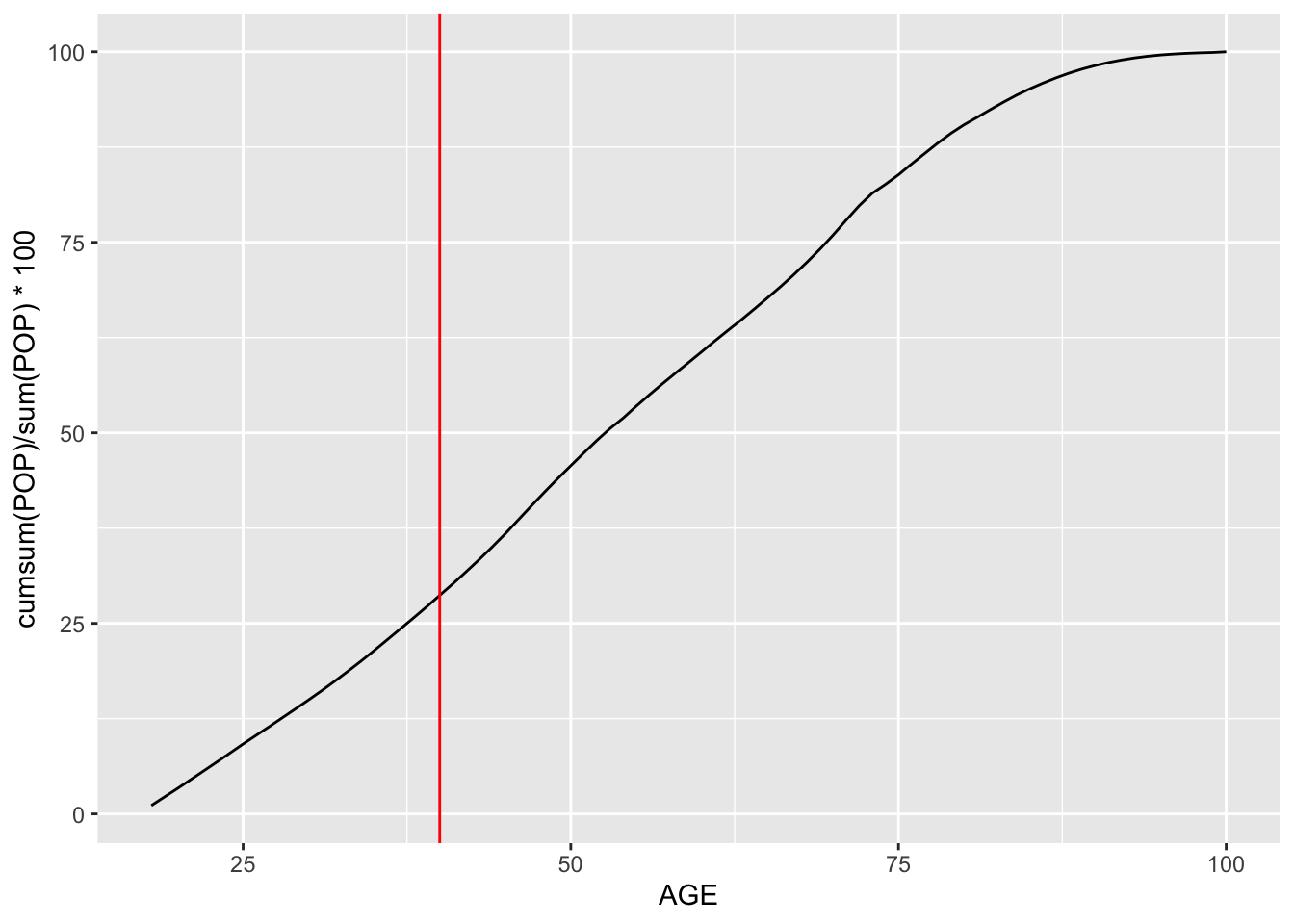

E.4 Population Pyramid

E.4.1 Population Pyramid of Japan or Other Countries

E.4.1.1 Japan

yr <- 2020
country <- "Japan"
filter(idb15, COUNTRY == country) %>% 
  select(YEAR, SEX, POP, AGE) %>%
  mutate(SEX = fct_recode(as_factor(SEX), "Both Sex" = "0", "Male" = "1", "Female" = "2"), POP = POP/1000) %>%
  filter(YEAR == yr, SEX != "Both Sex") %>% 
  ggplot(aes(x = AGE, y = ifelse(SEX == "Male", -POP, POP), fill = SEX)) + 
  geom_bar(stat = "identity") + 
  coord_flip() +
  labs(title = paste("Population Pyramid of", country, yr), 
       subtitle = "population unit in 1000") +
  scale_y_continuous(breaks = seq(-1000, 1000, 500), 
                     labels = as.character(c(1000, 500, 0, 500, 1000))) +
  ylab("Male vs Female") + 
  scale_fill_brewer(palette = "Set2")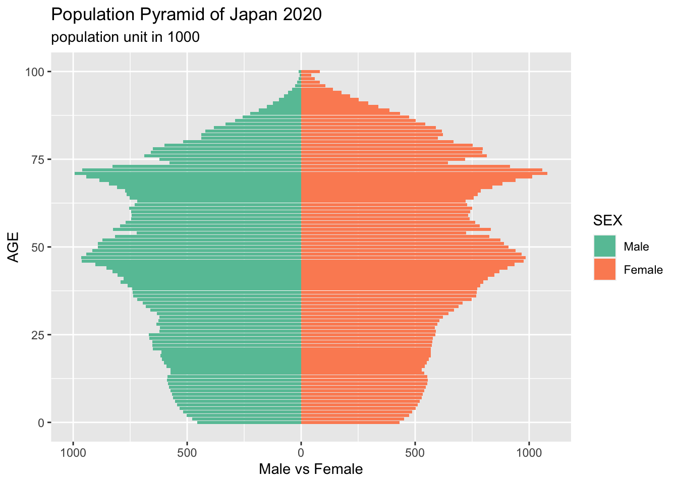

idb15 %>% filter(COUNTRY == country) %>% select(YEAR, SEX, POP, AGE) %>%
  mutate(SEX = as_factor(SEX)) %>% group_by(YEAR, SEX) %>% summarize(POPULATION = sum(POP)) %>%
  ggplot(aes(x = YEAR, y = POPULATION)) +
  geom_line(aes(color = SEX)) + 
  geom_vline(xintercept = 2020)

## `summarise()` has grouped output by 'YEAR'. You can override using the `.groups`
## argument.

E.4.1.2 Bangladesh

yr <- 2020
country <- "Bangladesh"
filter(idb15, COUNTRY == country) %>% 
  select(YEAR, SEX, POP, AGE) %>%
  mutate(SEX = fct_recode(as_factor(SEX), "Both Sex" = "0", "Male" = "1", "Female" = "2"), POP = POP/1000) %>%
  filter(YEAR == yr, SEX != "Both Sex") %>% 
  ggplot(aes(x = AGE, y = ifelse(SEX == "Male", -POP, POP), fill = SEX)) + 
  geom_bar(stat = "identity") + 
  coord_flip() +
  labs(title = paste("Population Pyramid of", country, yr), 
       subtitle = "population unit in 1000") +
  scale_y_continuous(breaks = seq(-1000, 1000, 500), 
                     labels = as.character(c(1000, 500, 0, 500, 1000))) +
  ylab("Male vs Female") + 
  scale_fill_brewer(palette = "Set2")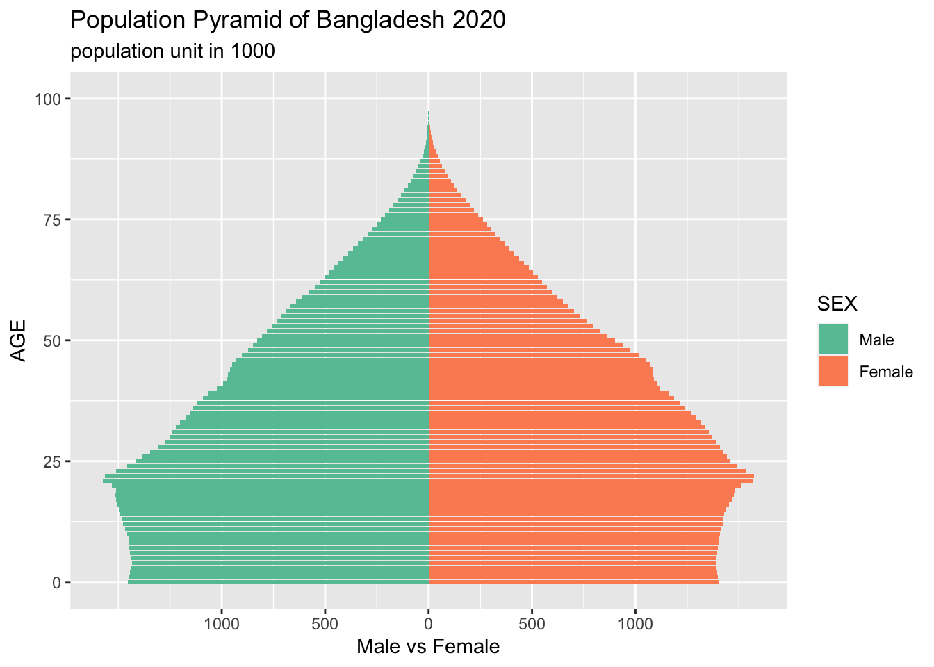

idb15 %>% filter(COUNTRY == country) %>% select(YEAR, SEX, POP, AGE) %>%
  mutate(SEX = as_factor(SEX)) %>% group_by(YEAR, SEX) %>% summarize(POPULATION = sum(POP)) %>%
  ggplot(aes(x = YEAR, y = POPULATION)) +
  geom_line(aes(color = SEX)) + 
  geom_vline(xintercept = 2020)

## `summarise()` has grouped output by 'YEAR'. You can override using the `.groups`
## argument.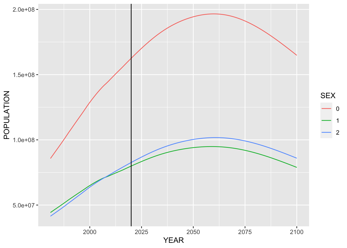

E.4.1.3 China

yr <- 2020
country <- "China"
filter(idb15, COUNTRY == country) %>% 
  select(YEAR, SEX, POP, AGE) %>%
  mutate(SEX = fct_recode(as_factor(SEX), "Both Sex" = "0", "Male" = "1", "Female" = "2"), POP = POP/1000) %>%
  filter(YEAR == yr, SEX != "Both Sex") %>% 
  ggplot(aes(x = AGE, y = ifelse(SEX == "Male", -POP, POP), fill = SEX)) + 
  geom_bar(stat = "identity") + 
  coord_flip() +
  labs(title = paste("Population Pyramid of", country, yr), 
       subtitle = "population unit in 1000") +
  scale_y_continuous(breaks = seq(-1000, 1000, 500), 
                     labels = as.character(c(1000, 500, 0, 500, 1000))) +
  ylab("Male vs Female") + 
  scale_fill_brewer(palette = "Set2")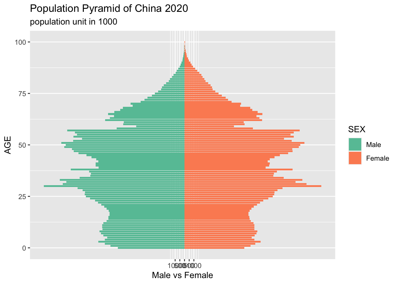

idb15 %>% filter(COUNTRY == country) %>% select(YEAR, SEX, POP, AGE) %>%
  mutate(SEX = as_factor(SEX)) %>% group_by(YEAR, SEX) %>% summarize(POPULATION = sum(POP)) %>%
  ggplot(aes(x = YEAR, y = POPULATION)) +
  geom_line(aes(color = SEX)) + 
  geom_vline(xintercept = 2020)

## `summarise()` has grouped output by 'YEAR'. You can override using the `.groups`
## argument.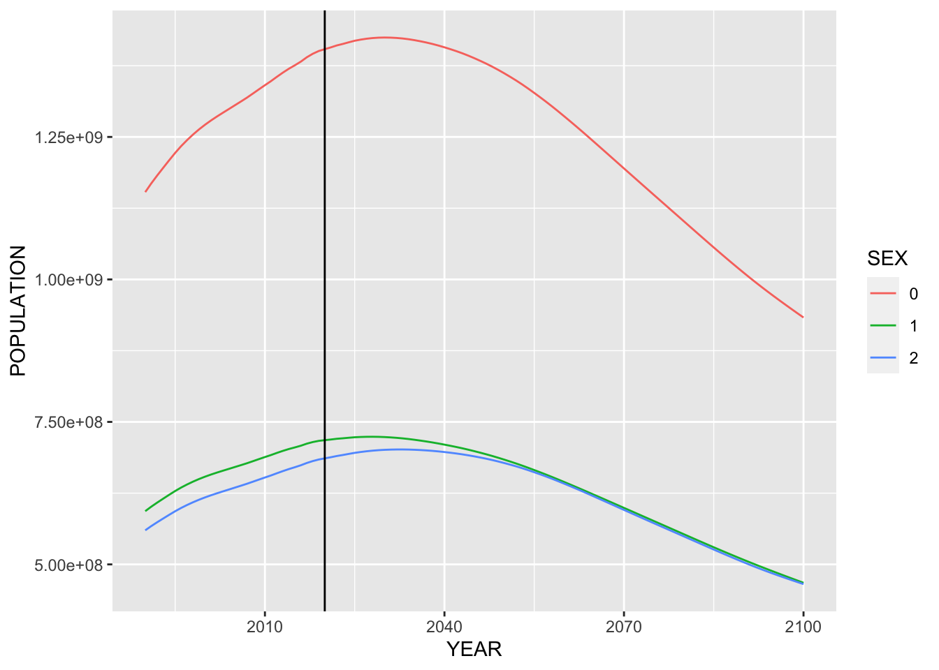

E.4.1.4 Germany

yr <- 2020
country <- "Germany"
filter(idb15, COUNTRY == country) %>% 
  select(YEAR, SEX, POP, AGE) %>%
  mutate(SEX = fct_recode(as_factor(SEX), "Both Sex" = "0", "Male" = "1", "Female" = "2"), POP = POP/1000) %>%
  filter(YEAR == yr, SEX != "Both Sex") %>% 
  ggplot(aes(x = AGE, y = ifelse(SEX == "Male", -POP, POP), fill = SEX)) + 
  geom_bar(stat = "identity") + 
  coord_flip() +
  labs(title = paste("Population Pyramid of", country, yr), 
       subtitle = "population unit in 1000") +
  scale_y_continuous(breaks = seq(-1000, 1000, 500), 
                     labels = as.character(c(1000, 500, 0, 500, 1000))) +
  ylab("Male vs Female") + 
  scale_fill_brewer(palette = "Set2")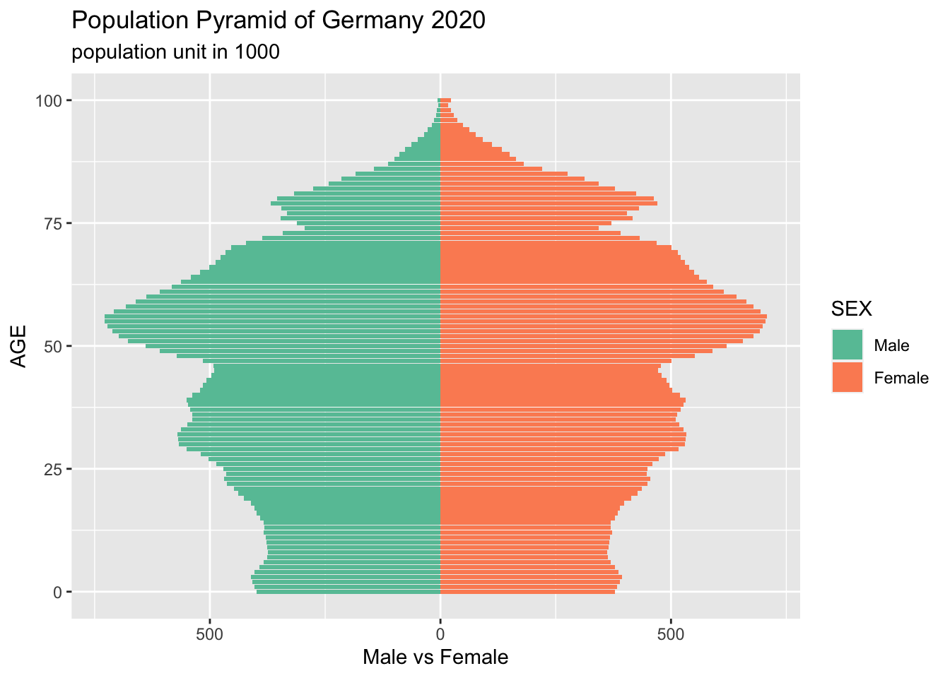

idb15 %>% filter(COUNTRY == country) %>% select(YEAR, SEX, POP, AGE) %>%
  mutate(SEX = as_factor(SEX)) %>% group_by(YEAR, SEX) %>% summarize(POPULATION = sum(POP)) %>%
  ggplot(aes(x = YEAR, y = POPULATION)) +
  geom_line(aes(color = SEX)) + 
  geom_vline(xintercept = 2020)

## `summarise()` has grouped output by 'YEAR'. You can override using the `.groups`
## argument.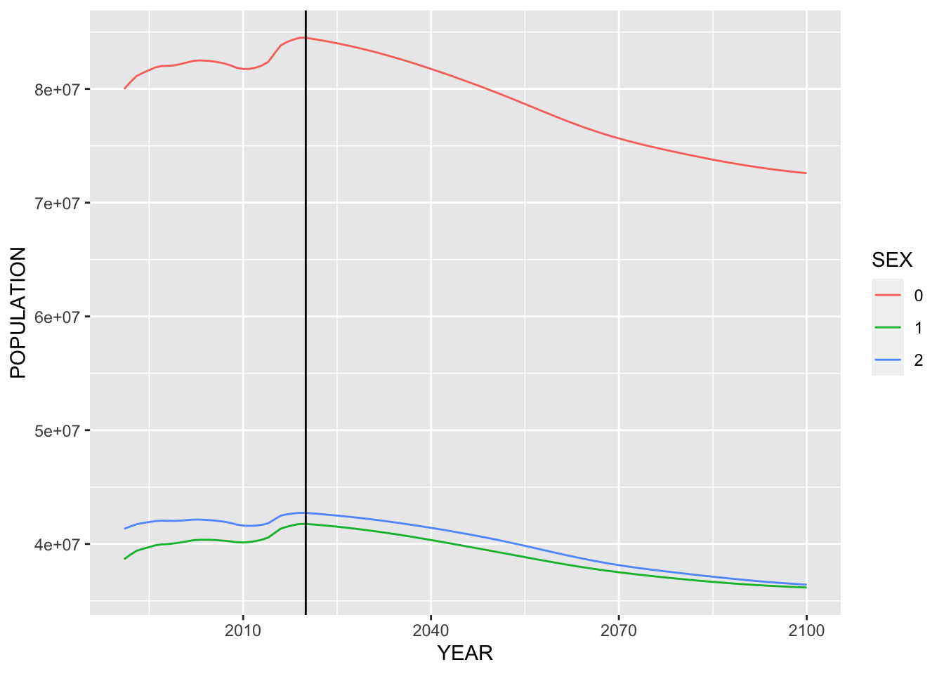

E.4.1.5 France

yr <- 2020
country <- "France"
filter(idb15, COUNTRY == country) %>% 
  select(YEAR, SEX, POP, AGE) %>%
  mutate(SEX = fct_recode(as_factor(SEX), "Both Sex" = "0", "Male" = "1", "Female" = "2"), POP = POP/1000) %>%
  filter(YEAR == yr, SEX != "Both Sex") %>% 
  ggplot(aes(x = AGE, y = ifelse(SEX == "Male", -POP, POP), fill = SEX)) + 
  geom_bar(stat = "identity") + 
  coord_flip() +
  labs(title = paste("Population Pyramid of", country, yr), 
       subtitle = "population unit in 1000") +
  scale_y_continuous(breaks = seq(-1000, 1000, 500), 
                     labels = as.character(c(1000, 500, 0, 500, 1000))) +
  ylab("Male vs Female") + 
  scale_fill_brewer(palette = "Set2")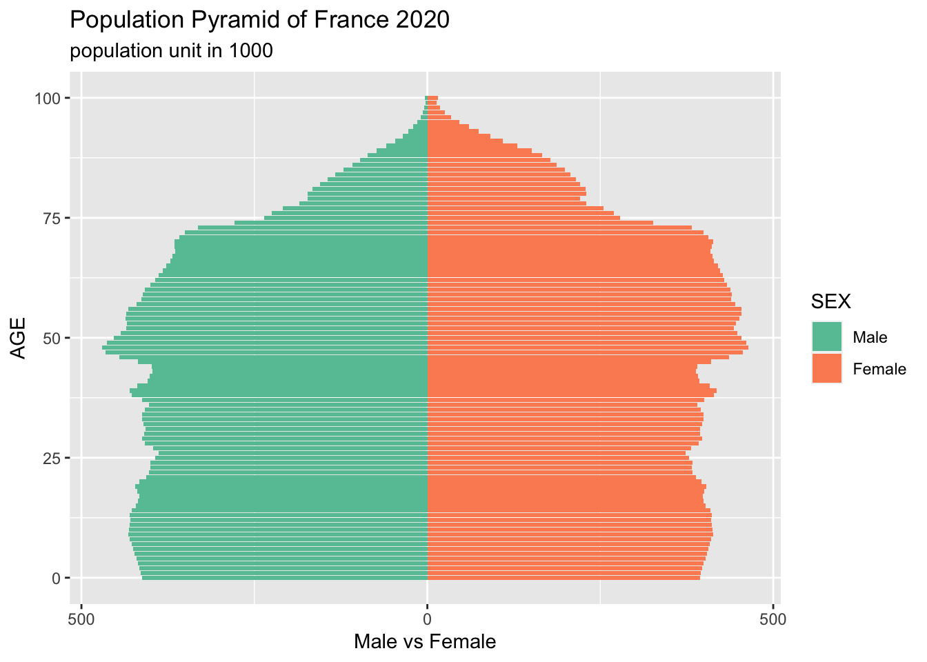

idb15 %>% filter(COUNTRY == country) %>% select(YEAR, SEX, POP, AGE) %>%
  mutate(SEX = as_factor(SEX)) %>% group_by(YEAR, SEX) %>% summarize(POPULATION = sum(POP)) %>%
  ggplot(aes(x = YEAR, y = POPULATION)) +
  geom_line(aes(color = SEX)) + 
  geom_vline(xintercept = 2020)

## `summarise()` has grouped output by 'YEAR'. You can override using the `.groups`
## argument.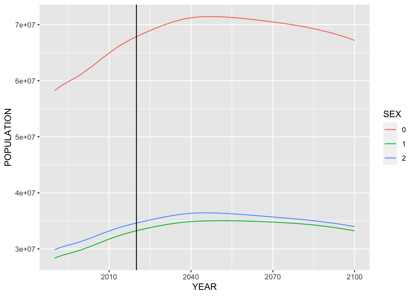

E.4.1.6 United Kingdom

yr <- 2020
country <- "United Kingdom"
filter(idb15, COUNTRY == country) %>% 
  select(YEAR, SEX, POP, AGE) %>%
  mutate(SEX = fct_recode(as_factor(SEX), "Both Sex" = "0", "Male" = "1", "Female" = "2"), POP = POP/1000) %>%
  filter(YEAR == yr, SEX != "Both Sex") %>% 
  ggplot(aes(x = AGE, y = ifelse(SEX == "Male", -POP, POP), fill = SEX)) + 
  geom_bar(stat = "identity") + 
  coord_flip() +
  labs(title = paste("Population Pyramid of", country, yr), 
       subtitle = "population unit in 1000") +
  scale_y_continuous(breaks = seq(-1000, 1000, 500), 
                     labels = as.character(c(1000, 500, 0, 500, 1000))) +
  ylab("Male vs Female") + 
  scale_fill_brewer(palette = "Set2")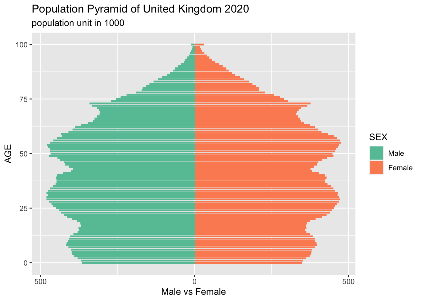

idb15 %>% filter(COUNTRY == country) %>% select(YEAR, SEX, POP, AGE) %>%
  mutate(SEX = as_factor(SEX)) %>% group_by(YEAR, SEX) %>% summarize(POPULATION = sum(POP)) %>%
  ggplot(aes(x = YEAR, y = POPULATION)) +
  geom_line(aes(color = SEX)) + 
  geom_vline(xintercept = 2020)

## `summarise()` has grouped output by 'YEAR'. You can override using the `.groups`
## argument.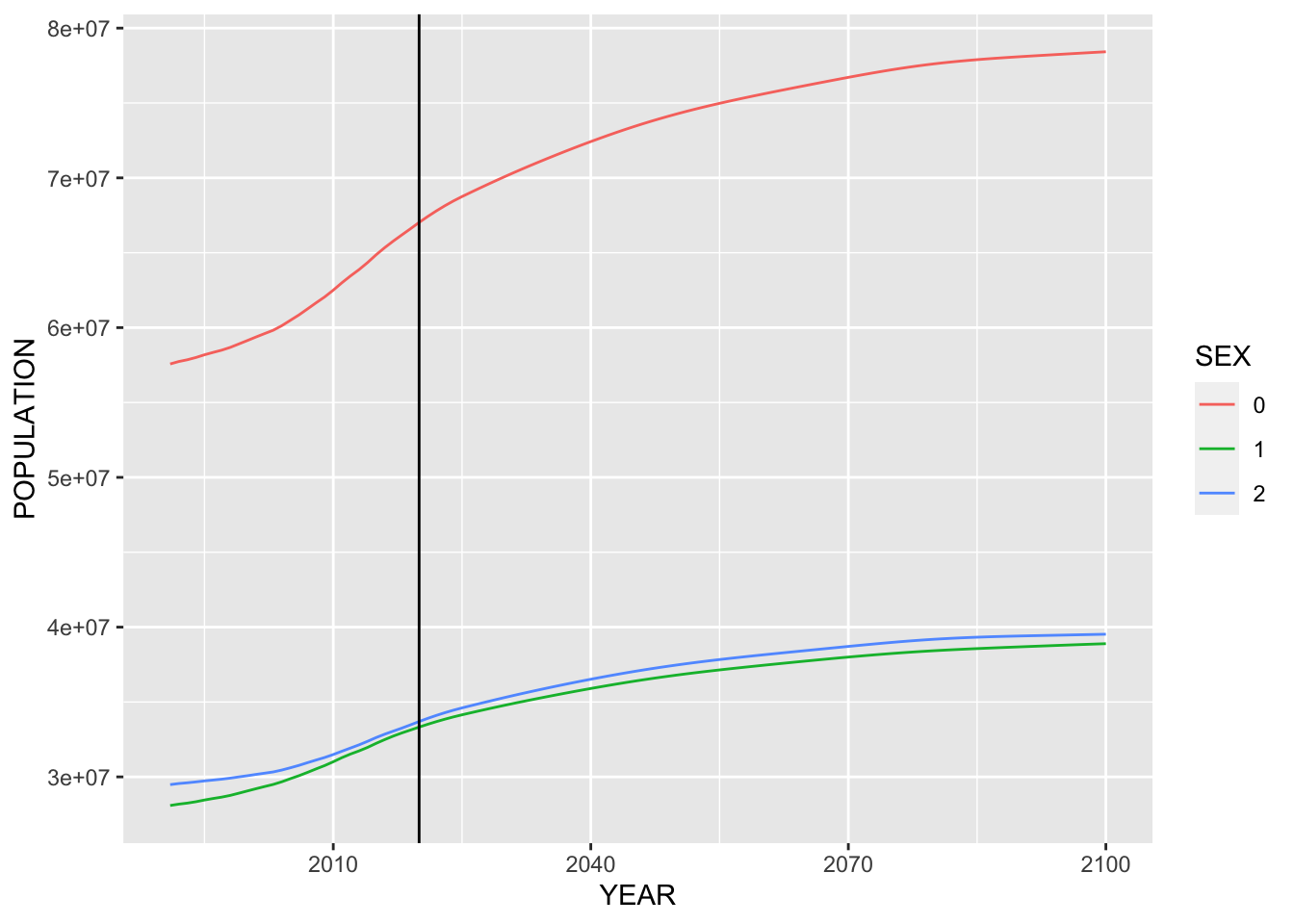

E.4.1.7 Indonesia

yr <- 2020
country <- "Indonesia"
filter(idb15, COUNTRY == country) %>% 
  select(YEAR, SEX, POP, AGE) %>%
  mutate(SEX = fct_recode(as_factor(SEX), "Both Sex" = "0", "Male" = "1", "Female" = "2"), POP = POP/1000) %>%
  filter(YEAR == yr, SEX != "Both Sex") %>% 
  ggplot(aes(x = AGE, y = ifelse(SEX == "Male", -POP, POP), fill = SEX)) + 
  geom_bar(stat = "identity") + 
  coord_flip() +
  labs(title = paste("Population Pyramid of", country, yr), 
       subtitle = "population unit in 1000") +
  scale_y_continuous(breaks = seq(-1000, 1000, 500), 
                     labels = as.character(c(1000, 500, 0, 500, 1000))) +
  ylab("Male vs Female") + 
  scale_fill_brewer(palette = "Set2")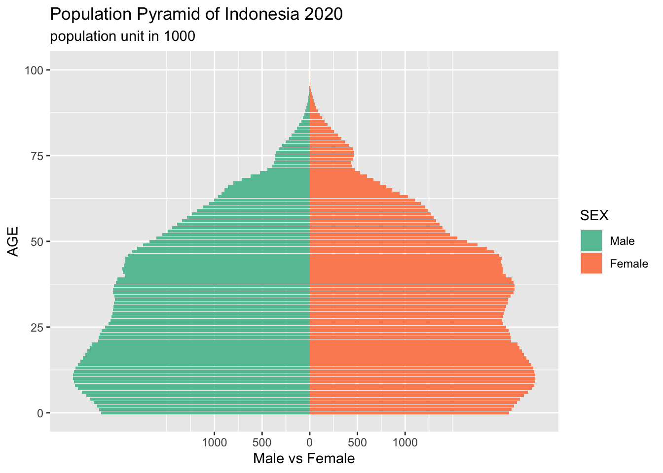

idb15 %>% filter(COUNTRY == country) %>% select(YEAR, SEX, POP, AGE) %>%
  mutate(SEX = as_factor(SEX)) %>% group_by(YEAR, SEX) %>% summarize(POPULATION = sum(POP)) %>%
  ggplot(aes(x = YEAR, y = POPULATION)) +
  geom_line(aes(color = SEX)) + 
  geom_vline(xintercept = 2020)

## `summarise()` has grouped output by 'YEAR'. You can override using the `.groups`
## argument.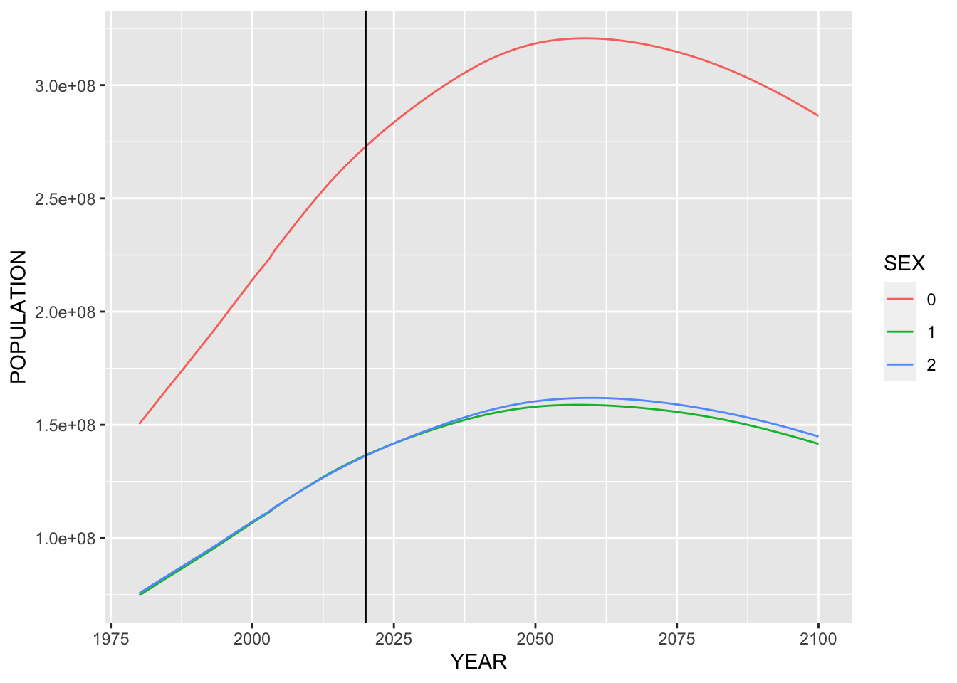

E.4.1.8 India

yr <- 2020
country <- "India"
filter(idb15, COUNTRY == country) %>% 
  select(YEAR, SEX, POP, AGE) %>%
  mutate(SEX = fct_recode(as_factor(SEX), "Both Sex" = "0", "Male" = "1", "Female" = "2"), POP = POP/1000) %>%
  filter(YEAR == yr, SEX != "Both Sex") %>% 
  ggplot(aes(x = AGE, y = ifelse(SEX == "Male", -POP, POP), fill = SEX)) + 
  geom_bar(stat = "identity") + 
  coord_flip() +
  labs(title = paste("Population Pyramid of", country, yr), 
       subtitle = "population unit in 1000") +
  scale_y_continuous(breaks = seq(-1000, 1000, 500), 
                     labels = as.character(c(1000, 500, 0, 500, 1000))) +
  ylab("Male vs Female") + 
  scale_fill_brewer(palette = "Set2")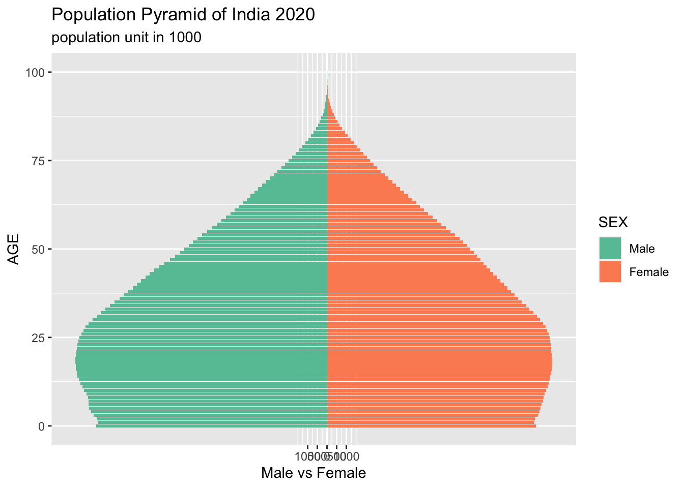

idb15 %>% filter(COUNTRY == country) %>% select(YEAR, SEX, POP, AGE) %>%
  mutate(SEX = as_factor(SEX)) %>% group_by(YEAR, SEX) %>% summarize(POPULATION = sum(POP)) %>%
  ggplot(aes(x = YEAR, y = POPULATION)) +
  geom_line(aes(color = SEX)) + 
  geom_vline(xintercept = 2020)

## `summarise()` has grouped output by 'YEAR'. You can override using the `.groups`
## argument.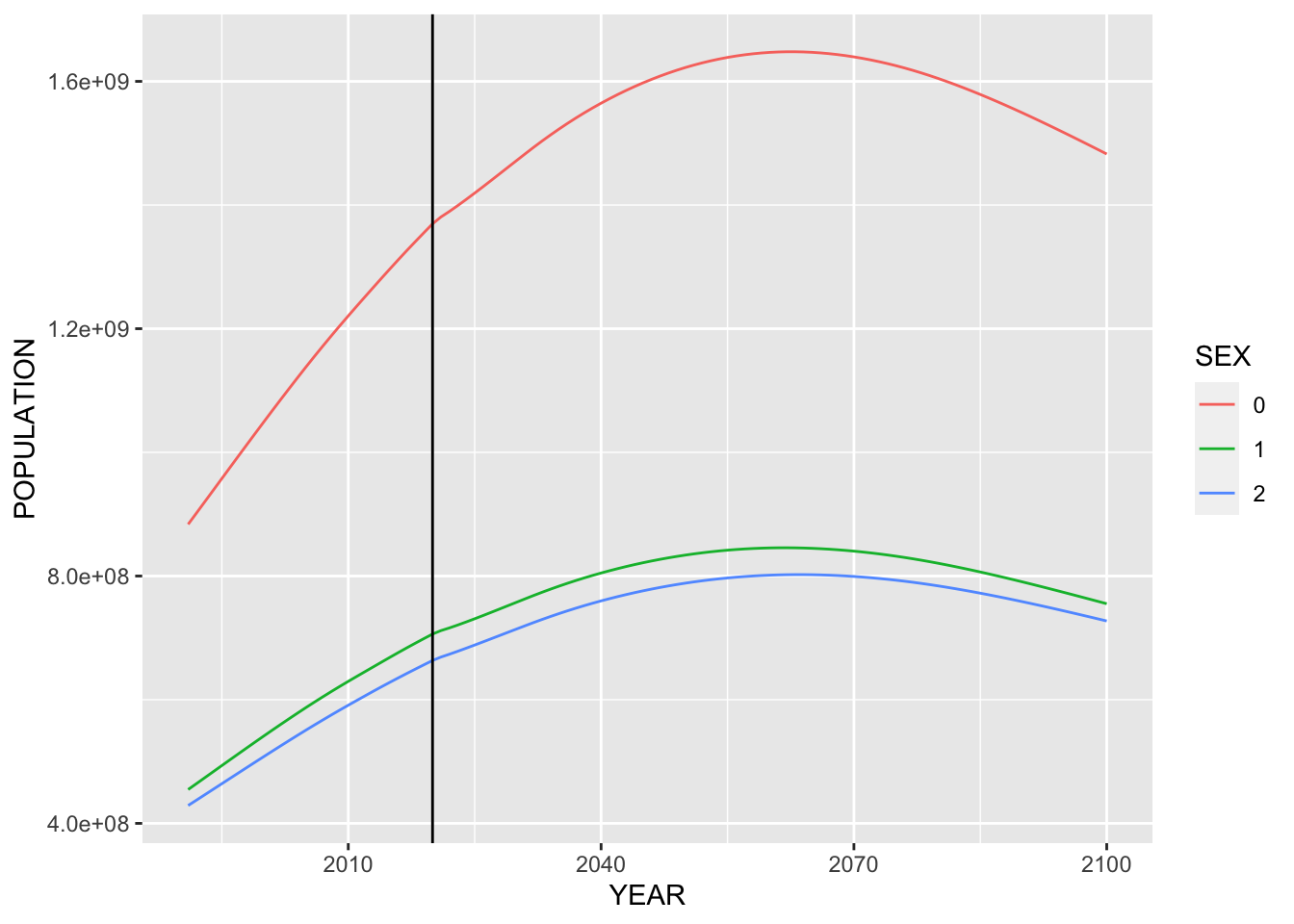

E.4.1.9 Korea, South

yr <- 2020
country <- "Korea, South"
filter(idb15, COUNTRY == country) %>% 
  select(YEAR, SEX, POP, AGE) %>%
  mutate(SEX = fct_recode(as_factor(SEX), "Both Sex" = "0", "Male" = "1", "Female" = "2"), POP = POP/1000) %>%
  filter(YEAR == yr, SEX != "Both Sex") %>% 
  ggplot(aes(x = AGE, y = ifelse(SEX == "Male", -POP, POP), fill = SEX)) + 
  geom_bar(stat = "identity") + 
  coord_flip() +
  labs(title = paste("Population Pyramid of", country, yr), 
       subtitle = "population unit in 1000") +
  scale_y_continuous(breaks = seq(-1000, 1000, 500), 
                     labels = as.character(c(1000, 500, 0, 500, 1000))) +
  ylab("Male vs Female") + 
  scale_fill_brewer(palette = "Set2")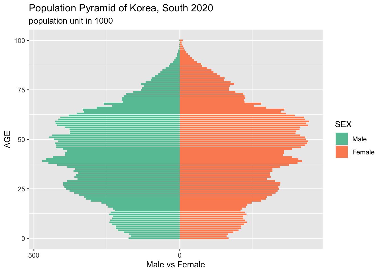

idb15 %>% filter(COUNTRY == country) %>% select(YEAR, SEX, POP, AGE) %>%
  mutate(SEX = as_factor(SEX)) %>% group_by(YEAR, SEX) %>% summarize(POPULATION = sum(POP)) %>%
  ggplot(aes(x = YEAR, y = POPULATION)) +
  geom_line(aes(color = SEX)) + 
  geom_vline(xintercept = 2020)

## `summarise()` has grouped output by 'YEAR'. You can override using the `.groups`
## argument.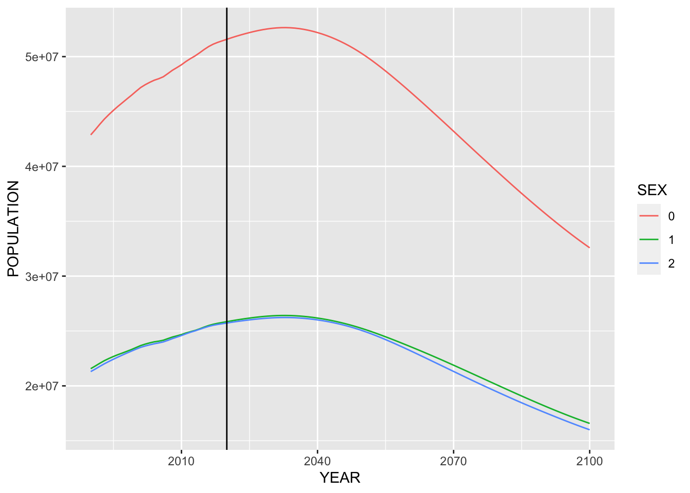

E.4.1.10 Sri Lanka

yr <- 2020
country <- "Sri Lanka"
filter(idb15, COUNTRY == country) %>% 
  select(YEAR, SEX, POP, AGE) %>%
  mutate(SEX = fct_recode(as_factor(SEX), "Both Sex" = "0", "Male" = "1", "Female" = "2"), POP = POP/1000) %>%
  filter(YEAR == yr, SEX != "Both Sex") %>% 
  ggplot(aes(x = AGE, y = ifelse(SEX == "Male", -POP, POP), fill = SEX)) + 
  geom_bar(stat = "identity") + 
  coord_flip() +
  labs(title = paste("Population Pyramid of", country, yr), 
       subtitle = "population unit in 1000") +
  scale_y_continuous(breaks = seq(-1000, 1000, 500), 
                     labels = as.character(c(1000, 500, 0, 500, 1000))) +
  ylab("Male vs Female") + 
  scale_fill_brewer(palette = "Set2")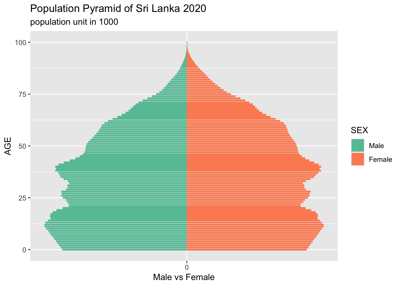

idb15 %>% filter(COUNTRY == country) %>% select(YEAR, SEX, POP, AGE) %>%
  mutate(SEX = as_factor(SEX)) %>% group_by(YEAR, SEX) %>% summarize(POPULATION = sum(POP)) %>%
  ggplot(aes(x = YEAR, y = POPULATION)) +
  geom_line(aes(color = SEX)) + 
  geom_vline(xintercept = 2020)

## `summarise()` has grouped output by 'YEAR'. You can override using the `.groups`
## argument.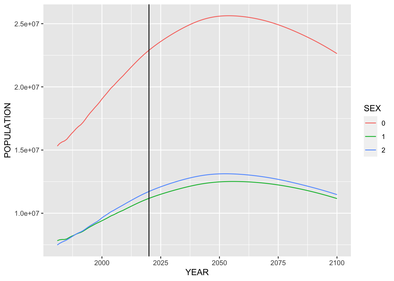

E.4.1.11 Malaysia

yr <- 2020
country <- "Malaysia"
filter(idb15, COUNTRY == country) %>% 
  select(YEAR, SEX, POP, AGE) %>%
  mutate(SEX = fct_recode(as_factor(SEX), "Both Sex" = "0", "Male" = "1", "Female" = "2"), POP = POP/1000) %>%
  filter(YEAR == yr, SEX != "Both Sex") %>% 
  ggplot(aes(x = AGE, y = ifelse(SEX == "Male", -POP, POP), fill = SEX)) + 
  geom_bar(stat = "identity") + 
  coord_flip() +
  labs(title = paste("Population Pyramid of", country, yr), 
       subtitle = "population unit in 1000") +
  scale_y_continuous(breaks = seq(-1000, 1000, 500), 
                     labels = as.character(c(1000, 500, 0, 500, 1000))) +
  ylab("Male vs Female") + 
  scale_fill_brewer(palette = "Set2")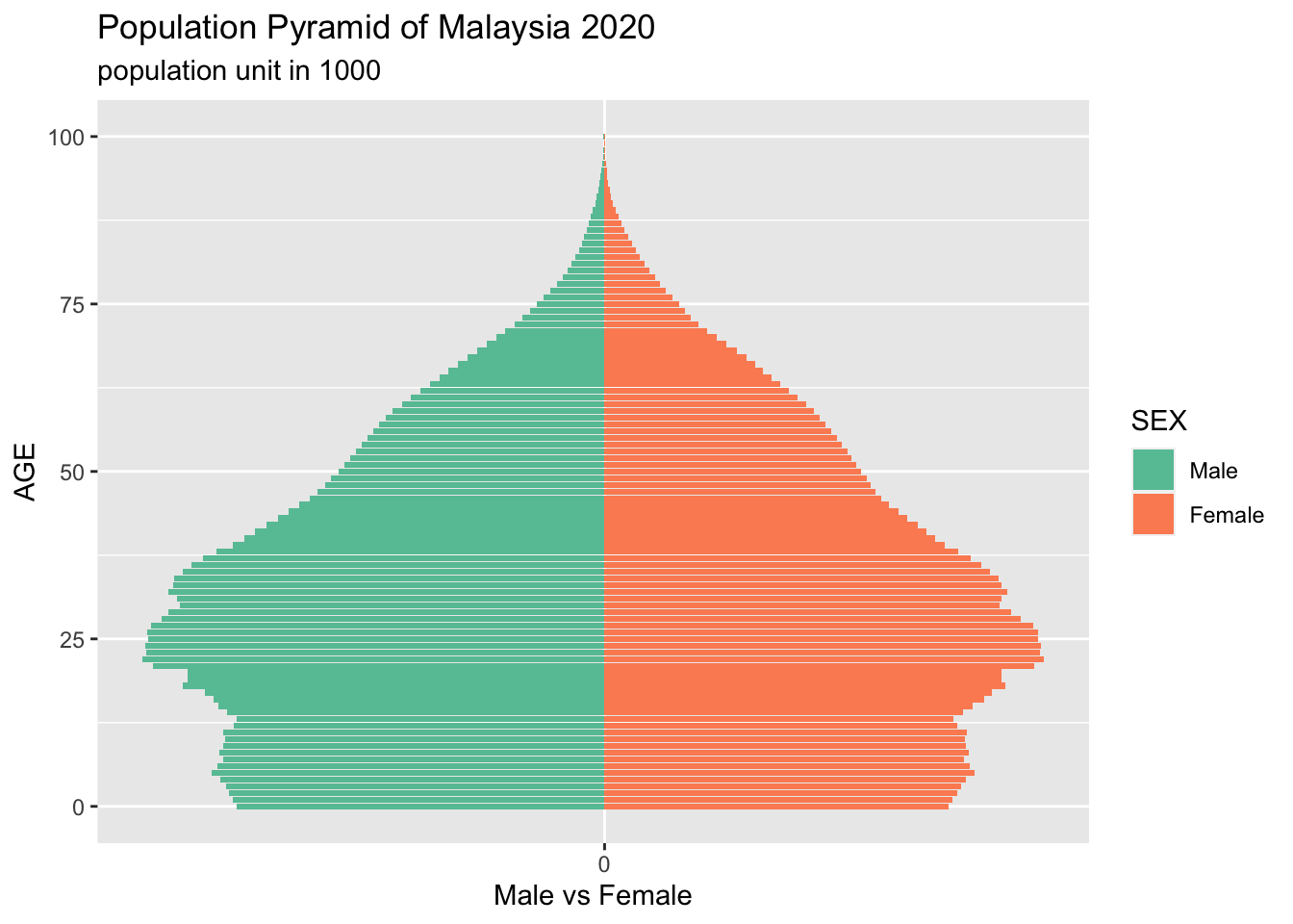

idb15 %>% filter(COUNTRY == country) %>% select(YEAR, SEX, POP, AGE) %>%
  mutate(SEX = as_factor(SEX)) %>% group_by(YEAR, SEX) %>% summarize(POPULATION = sum(POP)) %>%
  ggplot(aes(x = YEAR, y = POPULATION)) +
  geom_line(aes(color = SEX)) + 
  geom_vline(xintercept = 2020)

## `summarise()` has grouped output by 'YEAR'. You can override using the `.groups`
## argument.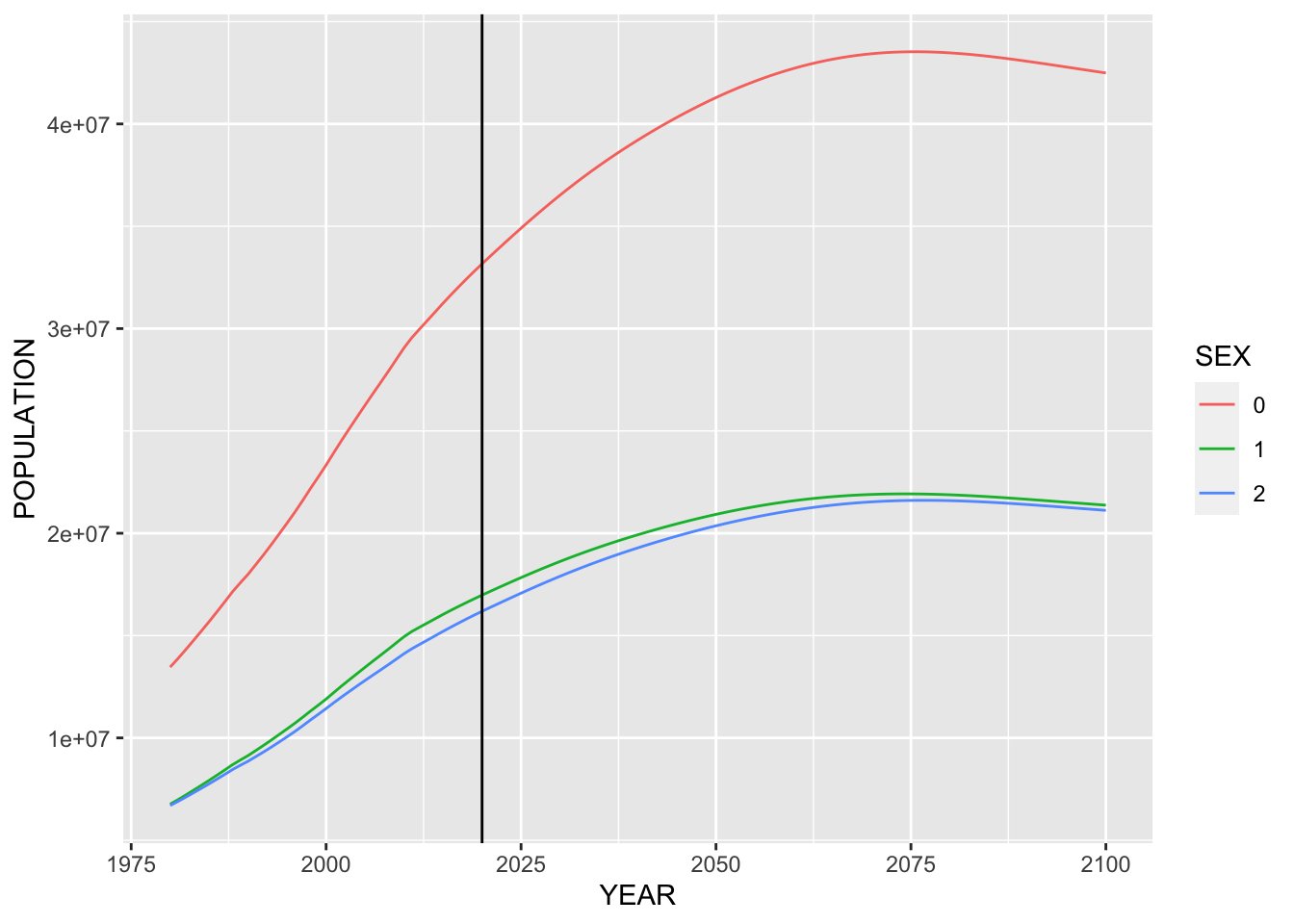

E.4.1.12 Philippines

yr <- 2020
country <- "Philippines"
filter(idb15, COUNTRY == country) %>% 
  select(YEAR, SEX, POP, AGE) %>%
  mutate(SEX = fct_recode(as_factor(SEX), "Both Sex" = "0", "Male" = "1", "Female" = "2"), POP = POP/1000) %>%
  filter(YEAR == yr, SEX != "Both Sex") %>% 
  ggplot(aes(x = AGE, y = ifelse(SEX == "Male", -POP, POP), fill = SEX)) + 
  geom_bar(stat = "identity") + 
  coord_flip() +
  labs(title = paste("Population Pyramid of", country, yr), 
       subtitle = "population unit in 1000") +
  scale_y_continuous(breaks = seq(-1000, 1000, 500), 
                     labels = as.character(c(1000, 500, 0, 500, 1000))) +
  ylab("Male vs Female") + 
  scale_fill_brewer(palette = "Set2")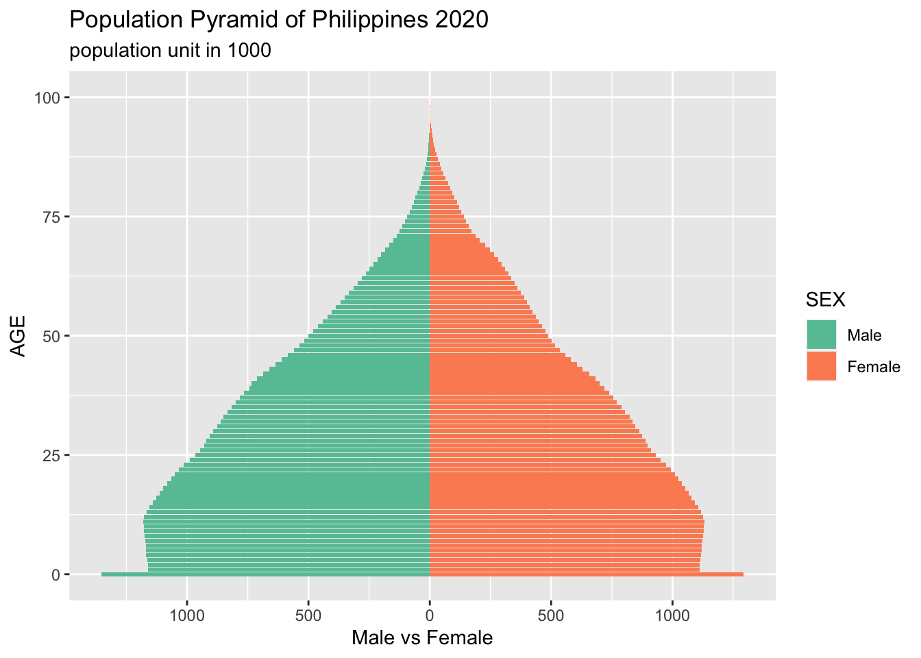

idb15 %>% filter(COUNTRY == country) %>% select(YEAR, SEX, POP, AGE) %>%
  mutate(SEX = as_factor(SEX)) %>% group_by(YEAR, SEX) %>% summarize(POPULATION = sum(POP)) %>%
  ggplot(aes(x = YEAR, y = POPULATION)) +
  geom_line(aes(color = SEX)) + 
  geom_vline(xintercept = 2020)

## `summarise()` has grouped output by 'YEAR'. You can override using the `.groups`
## argument.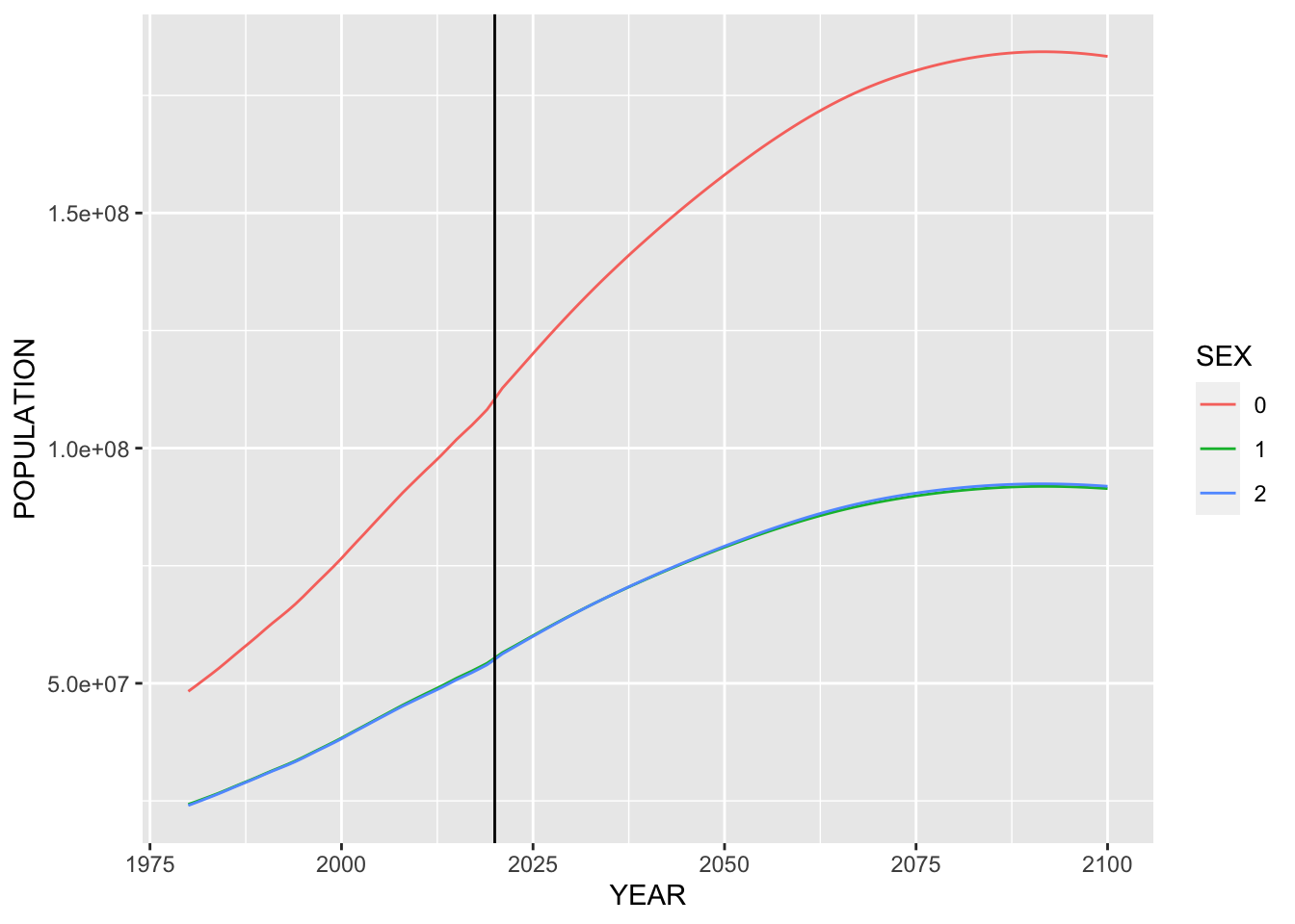

E.4.1.13 Thailand

yr <- 2020
country <- "Thailand"
filter(idb15, COUNTRY == country) %>% 
  select(YEAR, SEX, POP, AGE) %>%
  mutate(SEX = fct_recode(as_factor(SEX), "Both Sex" = "0", "Male" = "1", "Female" = "2"), POP = POP/1000) %>%
  filter(YEAR == yr, SEX != "Both Sex") %>% 
  ggplot(aes(x = AGE, y = ifelse(SEX == "Male", -POP, POP), fill = SEX)) + 
  geom_bar(stat = "identity") + 
  coord_flip() +
  labs(title = paste("Population Pyramid of", country, yr), 
       subtitle = "population unit in 1000") +
  scale_y_continuous(breaks = seq(-1000, 1000, 500), 
                     labels = as.character(c(1000, 500, 0, 500, 1000))) +
  ylab("Male vs Female") + 
  scale_fill_brewer(palette = "Set2")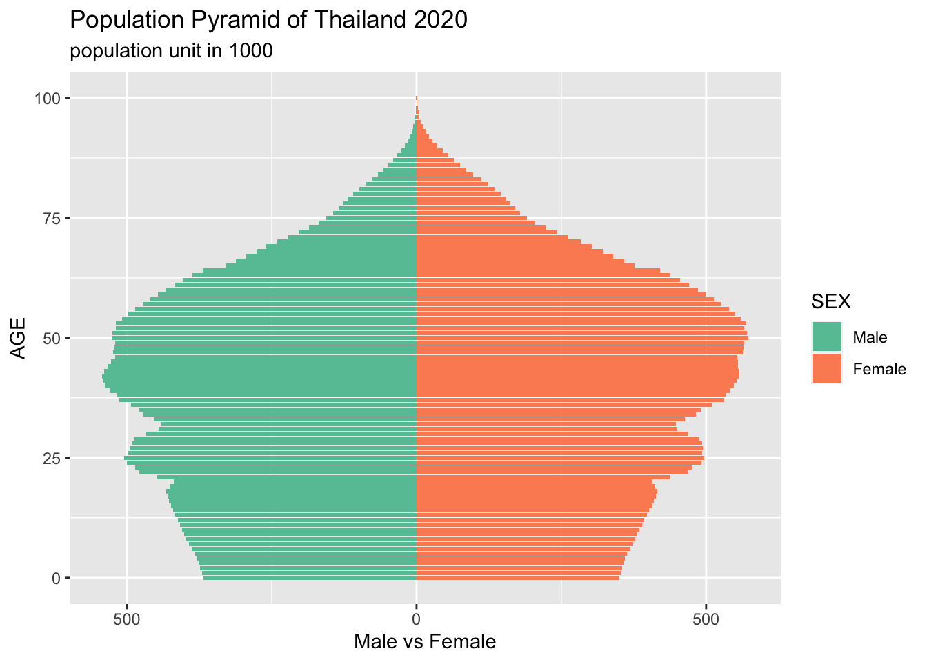

idb15 %>% filter(COUNTRY == country) %>% select(YEAR, SEX, POP, AGE) %>%
  mutate(SEX = as_factor(SEX)) %>% group_by(YEAR, SEX) %>% summarize(POPULATION = sum(POP)) %>%
  ggplot(aes(x = YEAR, y = POPULATION)) +
  geom_line(aes(color = SEX)) + 
  geom_vline(xintercept = 2020)

## `summarise()` has grouped output by 'YEAR'. You can override using the `.groups`
## argument.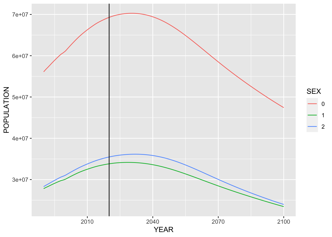

E.4.1.14 United States

yr <- 2020
country <- "United States"
filter(idb15, COUNTRY == country) %>% 
  select(YEAR, SEX, POP, AGE) %>%
  mutate(SEX = fct_recode(as_factor(SEX), "Both Sex" = "0", "Male" = "1", "Female" = "2"), POP = POP/1000) %>%
  filter(YEAR == yr, SEX != "Both Sex") %>% 
  ggplot(aes(x = AGE, y = ifelse(SEX == "Male", -POP, POP), fill = SEX)) + 
  geom_bar(stat = "identity") + 
  coord_flip() +
  labs(title = paste("Population Pyramid of", country, yr), 
       subtitle = "population unit in 1000") +
  scale_y_continuous(breaks = seq(-1000, 1000, 500), 
                     labels = as.character(c(1000, 500, 0, 500, 1000))) +
  ylab("Male vs Female") + 
  scale_fill_brewer(palette = "Set2")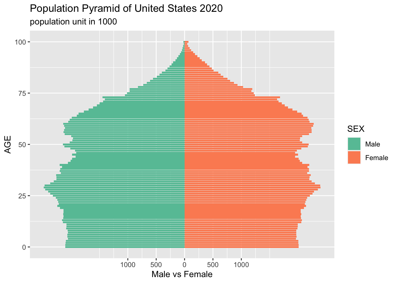

idb15 %>% filter(COUNTRY == country) %>% select(YEAR, SEX, POP, AGE) %>%
  mutate(SEX = as_factor(SEX)) %>% group_by(YEAR, SEX) %>% summarize(POPULATION = sum(POP)) %>%
  ggplot(aes(x = YEAR, y = POPULATION)) +
  geom_line(aes(color = SEX)) + 
  geom_vline(xintercept = 2020)

## `summarise()` has grouped output by 'YEAR'. You can override using the `.groups`
## argument.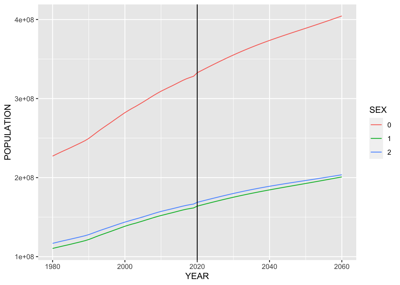

E.4.1.15 Vietnam

yr <- 2020
country <- "Vietnam"
filter(idb15, COUNTRY == country) %>% 
  select(YEAR, SEX, POP, AGE) %>%
  mutate(SEX = fct_recode(as_factor(SEX), "Both Sex" = "0", "Male" = "1", "Female" = "2"), POP = POP/1000) %>%
  filter(YEAR == yr, SEX != "Both Sex") %>% 
  ggplot(aes(x = AGE, y = ifelse(SEX == "Male", -POP, POP), fill = SEX)) + 
  geom_bar(stat = "identity") + 
  coord_flip() +
  labs(title = paste("Population Pyramid of", country, yr), 
       subtitle = "population unit in 1000") +
  scale_y_continuous(breaks = seq(-1000, 1000, 500), 
                     labels = as.character(c(1000, 500, 0, 500, 1000))) +
  ylab("Male vs Female") + 
  scale_fill_brewer(palette = "Set2")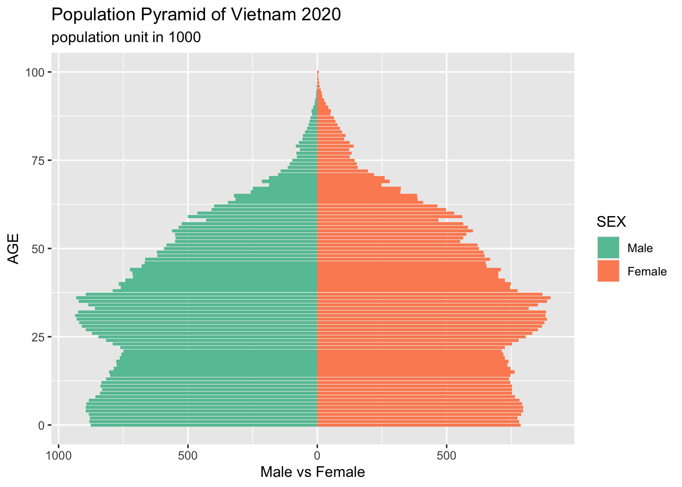

idb15 %>% filter(COUNTRY == country) %>% select(YEAR, SEX, POP, AGE) %>%
  mutate(SEX = as_factor(SEX)) %>% group_by(YEAR, SEX) %>% summarize(POPULATION = sum(POP)) %>%
  ggplot(aes(x = YEAR, y = POPULATION)) +
  geom_line(aes(color = SEX)) + 
  geom_vline(xintercept = 2020)

## `summarise()` has grouped output by 'YEAR'. You can override using the `.groups`
## argument.

E.4.1.16 Project

Try Other Countries or Regions Using CLASS.xlsx of United Nations

End of Analysis