Chapter 2 Exploratory Data Analysis (EDA) 1

2.1 R with R Studio and/or R Studio.cloud

2.1.1 Course Contents

  1. 2020-12-08: Introduction: About the course
    - An introduction to open and public data, and data science
  2. 2020-12-15: Exploratory Data Analysis (EDA) 1 [lead by hs]
    - R Basics with RStudio and/or RStudio.cloud; R Script, swirl
  3. 2021-12-22: Exploratory Data Analysis (EDA) 2 [lead by hs]
    - R Markdown; Introduction to tidyverse; RStudio Primers
  4. 2022-01-12: Exploratory Data Analysis (EDA) 3 [lead by hs]
    - Introduction to tidyverse; Public Data, WDI, etc
  5. 2022-01-19: Exploratory Data Analysis (EDA) 4 [lead by hs]
    - Introduction to tidyverse; WDI, UN, WHO, etc
  6. 2022-01-26: Exploratory Data Analysis (EDA) 5 [lead by hs]
    - Introduction to tidyverse; WDI, OECD, US gov, etc
  7. 2022-02-02: Inference Statistics 1
  8. 2022-02-09: Inference Statistics 2
  9. 2022-02-16: Inference Statistics 3
  10. 2022-02-23: Project Presentation

2.1.2 Learning Resources, I

2.1.2.1 Textbooks

“R for Data Science” by Hadley Wickham and Garrett Grolemund:

“R for Data Science: Exercise Solutions” by Jeffrey B. Arnold

2.1.2.2 Other Resources (MOOCs)

2.1.3 EDA1: Contents

  • What is R?

  • Why R?

    • the First Example
  • What is R Studio and R Studio Cloud?

  • Installation of R and R Studio
     

  • R Studio Basics

  • R Studio Cloud Basics

    • Project, R Console
  • R Basics using an R Script

  • {swirl}: Learn R, in R

  • EDA: Coronavirus, the first example

  • Assignment 1 and Assignment 2 in Moodle

2.1.4 What is R?

2.1.4.1 R (programming language), Wikipedia

  • R is a programming language and free software environment for statistical computing and graphics supported by the R Foundation for Statistical Computing.

  • The R language is widely used among statisticians and data miners for developing statistical software and data analysis.

  • A GNU package, the official R software environment is written primarily in C, Fortran, and R itself (thus, it is partially self-hosting) and is freely available under the GNU General Public License.

2.1.4.2 History of R and more

“R Programming for Data Science” by Roger Peng

2.1.5 Why R? – Responses by Hadley Wickham

2.1.5.1 r4ds: R is a great place to start your data science journey because

  • R is an environment designed from the ground up to support data science.
  • R is not just a programming language, but it is also an interactive environment for doing data science.
  • To support interaction, R is a much more flexible language than many of its peers.

2.1.5.2 Why R today?

When you talk about choosing programming languages, I always say you shouldn’t pick them based on technical merits, but rather pick them based on the community. And I think the R community is like really, really strong, vibrant, free, welcoming, and embraces a wide range of domains. So, if there are like people like you using R, then your life is going to be much easier. That’s the first reason.

Interview: “Advice to Young (and Old) Programmers, H. Wickham”

2.1.6 The First Example

plot(cars)
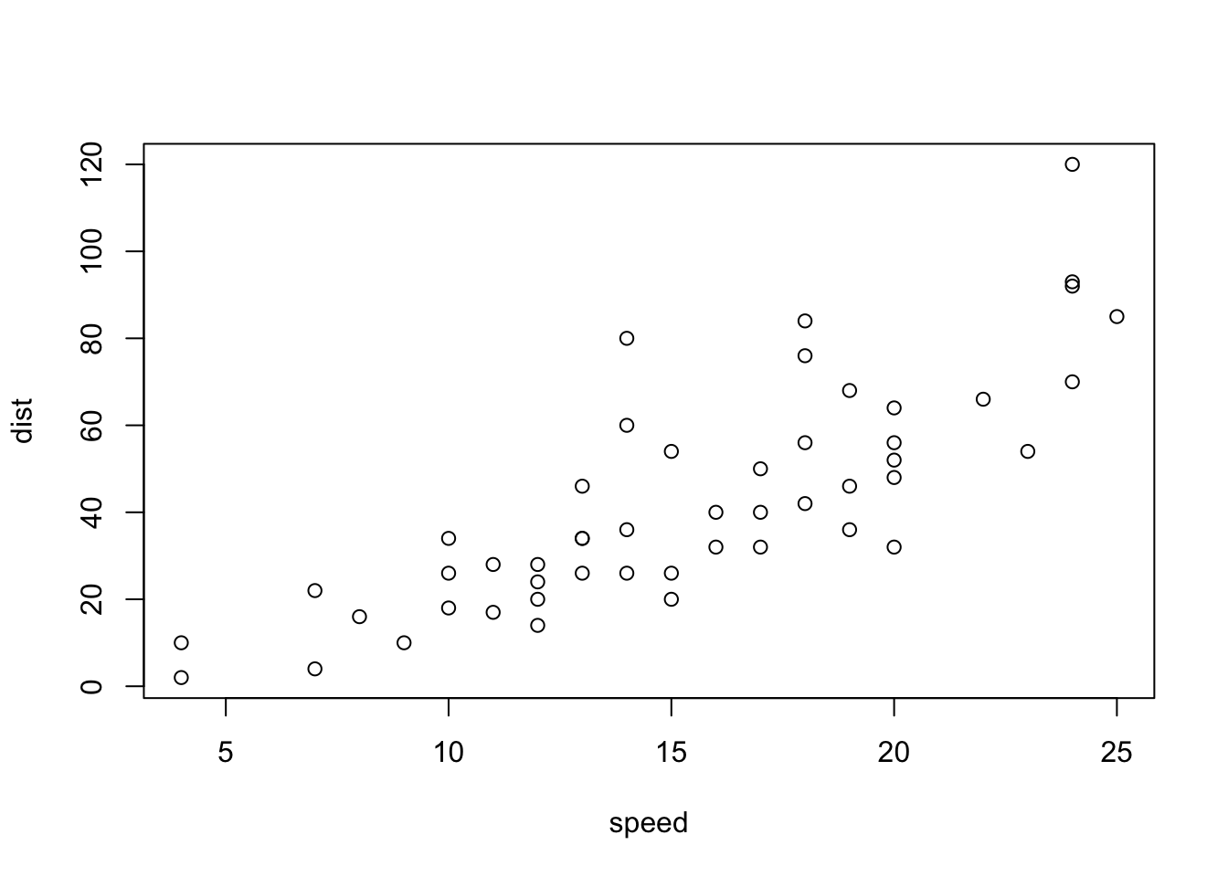
plot(cars) # cars: Speed and Stopping Distances of Cars
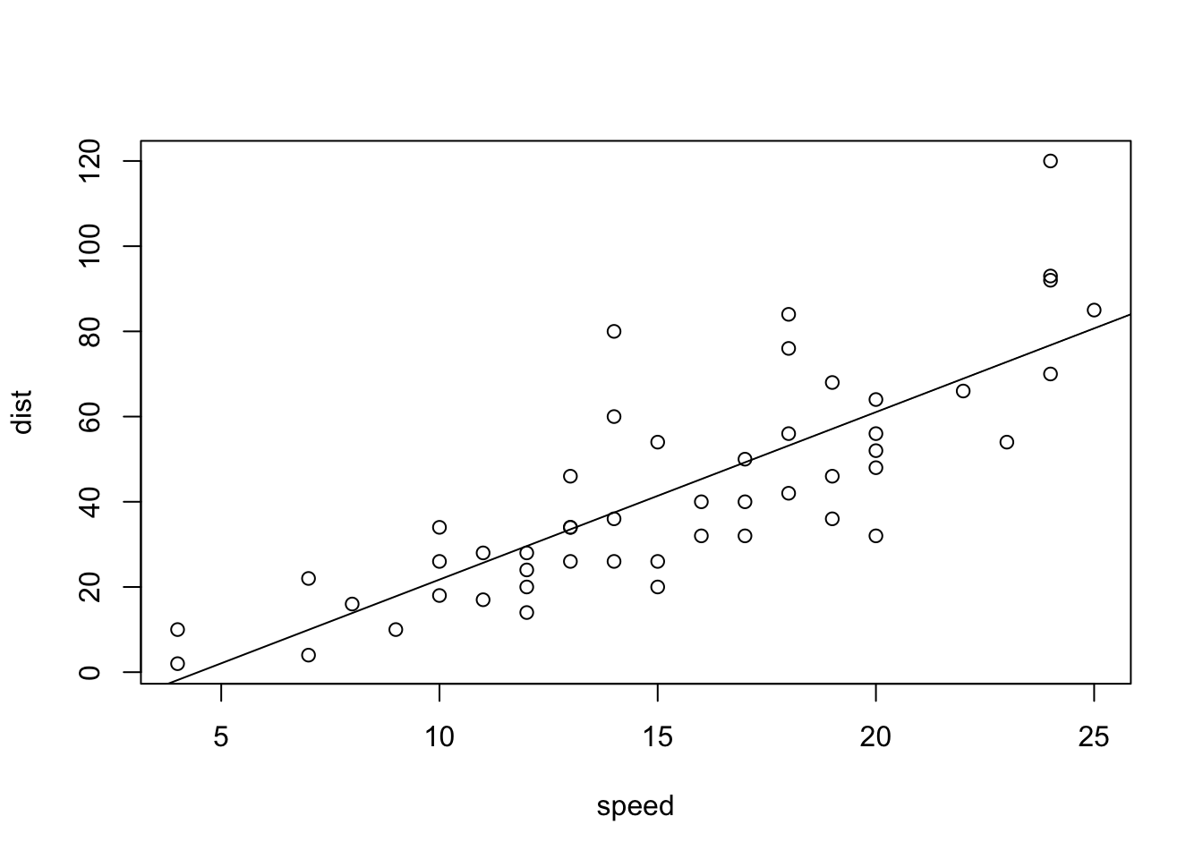
abline(lm(cars$dist~cars$speed))

head(cars)
##   speed dist
## 1     4    2
## 2     4   10
## 3     7    4
## 4     7   22
## 5     8   16
## 6     9   10
summary(cars)
##      speed           dist       
##  Min.   : 4.0   Min.   :  2.00  
##  1st Qu.:12.0   1st Qu.: 26.00  
##  Median :15.0   Median : 36.00  
##  Mean   :15.4   Mean   : 42.98  
##  3rd Qu.:19.0   3rd Qu.: 56.00  
##  Max.   :25.0   Max.   :120.00
summary(lm(cars$dist~cars$speed))
## 
## Call:
## lm(formula = cars$dist ~ cars$speed)
## 
## Residuals:
##     Min      1Q  Median      3Q     Max 
## -29.069  -9.525  -2.272   9.215  43.201 
## 
## Coefficients:
##             Estimate Std. Error t value Pr(>|t|)    
## (Intercept) -17.5791     6.7584  -2.601   0.0123 *  
## cars$speed    3.9324     0.4155   9.464 1.49e-12 ***
## ---
## Signif. codes:  0 '***' 0.001 '**' 0.01 '*' 0.05 '.' 0.1 ' ' 1
## 
## Residual standard error: 15.38 on 48 degrees of freedom
## Multiple R-squared:  0.6511, Adjusted R-squared:  0.6438 
## F-statistic: 89.57 on 1 and 48 DF,  p-value: 1.49e-12

2.1.7 What is RStudio? https://rstudio.com

RStudio is an integrated development environment, or IDE, for R programming.

2.1.7.1 R Studio (Wikipedia)

RStudio is an integrated development environment (IDE) for R, a programming language for statistical computing and graphics. It is available in two formats: RStudio Desktop is a regular desktop application while RStudio Server runs on a remote server and allows accessing RStudio using a web browser.

2.1.7.2 R Studio Cloud https://rstudio.cloud

RStudio Cloud is a lightweight, cloud-based solution that allows anyone to do, share, teach and learn data science online.

2.1.8 Installation of R and R Studio

2.1.8.1 R Installation

To download R, go to CRAN, the comprehensive R archive network. CRAN is composed of a set of mirror servers distributed around the world and is used to distribute R and R packages. Don’t try and pick a mirror that’s close to you: instead use the cloud mirror, https://cloud.r-project.org, which automatically figures it out for you.

A new major version of R comes out once a year, and there are 2-3 minor releases each year. It’s a good idea to update regularly.

2.1.8.2 R Studio Installation

Download and install it from http://www.rstudio.com/download.

RStudio is updated a couple of times a year. When a new version is available, RStudio will let you know.

2.1.9 R Studio

2.1.9.1 The First Step

  1. Start R Studio Application
  2. Top Menu: File > New Project > New Directory > New Project > Directory name or Browse the directory and choose the parent directory you want to create the directory

2.1.9.2 When You Start the Project

  1. Go to the directory you created
  2. Double click _‘Directory Name’.Rproj

Or,

  1. Start R Studio
  2. File > Open Project (or choose from Recent Project)

In this way the working directory of the session is set to the project directory and R can search releted files without difficulty (getwd(), setwd())

2.1.10 R Studio Cloud

2.1.10.1 Cloud Free

  • Up to 15 projects total
  • 1 shared space (5 members and 10 projects max)
  • 15 project hours per month
  • Up to 1 GB RAM per project
  • Up to 1 CPU per project
  • Up to 1 hour background execution time

2.1.10.2 How to Start R Studio Cloud

  1. Go to https://rstudio.cloud/
  2. Sign Up: top right
  • Email address or Google account
  1. New Project: Project Name
  2. R Console

2.1.11 Let’s Try R Basics

2.1.11.1 R Basics

Let’s Try R on R Studio and/or R Studio Cloud

2.1.11.2 R Scripts

  1. Copy a script in Moodle: basics.R
  2. In RStudio (Workspace in RStudio.cloud, Project in RStudio) choose File > New File > R Script and paste it.
  3. Choose File > Save with a name; e.g. basics (.R will be added automatically)

2.1.11.3 Helpful Resources

2.1.12 More on R Script: Examples

2.1.12.1 R Scripts in Moodle

  • basics.R
  • coronavirus.R
  1. Copy a script in Moodle: {file name}.R
  2. In RStudio (Workspace in RStudio.cloud, Project in RStudio) choose File > New File > R Script and paste it.
  3. Choose File > Save with a name; e.g. {file names} (.R will be added automatically)

2.1.13 Practicum: R Studio Cloud (or R Studio) and R basics

2.1.13.1 Let’s Try R Basics

  • R Studio Cloud
    • Create an account
    • Create a Project
  • R Studio Basics
  • R Basics
  • basics.R

2.1.13.2 Basics.R

The script with the outputs.

#################
#
# basics.R
#
################
# 'Quick R' by DataCamp may be a handy reference: 
#     https://www.statmethods.net/management/index.html
# Cheat Sheet at RStudio: https://www.rstudio.com/resources/cheatsheets/
# Base R Cheat Sheet: https://github.com/rstudio/cheatsheets/raw/main/base-r.pdf
# To execute the line: Control + Enter (Window and Linux), Command + Enter (Mac)
## try your experiments on the console

## calculator

3 + 7
## [1] 10
### +, -, *, /, ^ (or **), %%, %/%

3 + 10 / 2
## [1] 8
3^2
## [1] 9
2^3
## [1] 8
2*2*2
## [1] 8
### assignment: <-, (=, ->, assign()) 

x <- 5

x 
## [1] 5
#### object_name <- value, '<-' shortcut: Alt (option) + '-' (hyphen or minus) 
#### Object names must start with a letter and can only contain letter, numbers, _ and .

this_is_a_long_name <- 5^3

this_is_a_long_name
## [1] 125
char_name <- "What is your name?"

char_name
## [1] "What is your name?"
#### Use 'tab completion' and 'up arrow'

### ls(): list of all assignments

ls()
## [1] "char_name"           "this_is_a_long_name" "x"
ls.str()
## char_name :  chr "What is your name?"
## this_is_a_long_name :  num 125
## x :  num 5
#### check Environment in the upper right pane

### (atomic) vectors

5:10
## [1]  5  6  7  8  9 10
a <- seq(5,10)

a
## [1]  5  6  7  8  9 10
b <- 5:10

identical(a,b)
## [1] TRUE
seq(5,10,2) # same ase seq(from = 5, to = 10, by = 2)
## [1] 5 7 9
c1 <- seq(0,100, by = 10)

c2 <- seq(0,100, length.out = 10)

c1
##  [1]   0  10  20  30  40  50  60  70  80  90 100
c2
##  [1]   0.00000  11.11111  22.22222  33.33333  44.44444  55.55556  66.66667
##  [8]  77.77778  88.88889 100.00000
length(c1)
## [1] 11
#### ? seq   ? length   ? identical

(die <- 1:6)
## [1] 1 2 3 4 5 6
zero_one <- c(0,1) # same as 0:1

die + zero_one # c(1,2,3,4,5,6) + c(0,1). re-use
## [1] 1 3 3 5 5 7
d1 <- rep(1:3,2) # repeat


d1
## [1] 1 2 3 1 2 3
die == d1
## [1]  TRUE  TRUE  TRUE FALSE FALSE FALSE
d2 <- as.character(die == d1)

d2
## [1] "TRUE"  "TRUE"  "TRUE"  "FALSE" "FALSE" "FALSE"
d3 <- as.numeric(die == d1)

d3
## [1] 1 1 1 0 0 0
### class() for class and typeof() for mode
### class of vectors: numeric, charcters, logical
### types of vectors: doubles, integers, characters, logicals (complex and raw)

typeof(d1); class(d1)
## [1] "integer"
## [1] "integer"
typeof(d2); class(d2)
## [1] "character"
## [1] "character"
typeof(d3); class(d3)
## [1] "double"
## [1] "numeric"
sqrt(2)
## [1] 1.414214
sqrt(2)^2
## [1] 2
sqrt(2)^2 - 2
## [1] 4.440892e-16
typeof(sqrt(2))
## [1] "double"
typeof(2)
## [1] "double"
typeof(2L)
## [1] "integer"
5 == c(5)
## [1] TRUE
length(5)
## [1] 1
### Subsetting

(A_Z <- LETTERS)
##  [1] "A" "B" "C" "D" "E" "F" "G" "H" "I" "J" "K" "L" "M" "N" "O" "P" "Q" "R" "S"
## [20] "T" "U" "V" "W" "X" "Y" "Z"
A_F <- A_Z[1:6]

A_F
## [1] "A" "B" "C" "D" "E" "F"
A_F[3]
## [1] "C"
A_F[c(3,5)]
## [1] "C" "E"
large <- die > 3

large
## [1] FALSE FALSE FALSE  TRUE  TRUE  TRUE
even <- die %in% c(2,4,6)

even
## [1] FALSE  TRUE FALSE  TRUE FALSE  TRUE
A_F[large]
## [1] "D" "E" "F"
A_F[even]
## [1] "B" "D" "F"
A_F[die < 4]
## [1] "A" "B" "C"
### Compare df with df1 <- data.frame(number = die, alphabet = A_F)
df <- data.frame(number = die, alphabet = A_F, stringsAsFactors = FALSE)

df
##   number alphabet
## 1      1        A
## 2      2        B
## 3      3        C
## 4      4        D
## 5      5        E
## 6      6        F
df$number
## [1] 1 2 3 4 5 6
df$alphabet
## [1] "A" "B" "C" "D" "E" "F"
df[3,2]
## [1] "C"
df[4,1]
## [1] 4
df[1]
##   number
## 1      1
## 2      2
## 3      3
## 4      4
## 5      5
## 6      6
class(df[1])
## [1] "data.frame"
class(df[[1]])
## [1] "integer"
identical(df[[1]], die)
## [1] TRUE
identical(df[1],die)
## [1] FALSE
####################
# The First Example
####################

plot(cars)

# Help

? cars

# cars is in the 'datasets' package

data()

# help(cars) does the same as ? cars
# You can use Help tab in the right bottom pane

help(plot)
## トピック 'plot' に対するヘルプが以下のパッケージ中にありました:
## 
##   Package               Library
##   graphics              /Library/Frameworks/R.framework/Versions/4.2/Resources/library
##   base                  /Library/Frameworks/R.framework/Resources/library
## 
## 
##  最初にマッチしたものを使っています ...
? par

head(cars)
##   speed dist
## 1     4    2
## 2     4   10
## 3     7    4
## 4     7   22
## 5     8   16
## 6     9   10
str(cars)
## 'data.frame':    50 obs. of  2 variables:
##  $ speed: num  4 4 7 7 8 9 10 10 10 11 ...
##  $ dist : num  2 10 4 22 16 10 18 26 34 17 ...
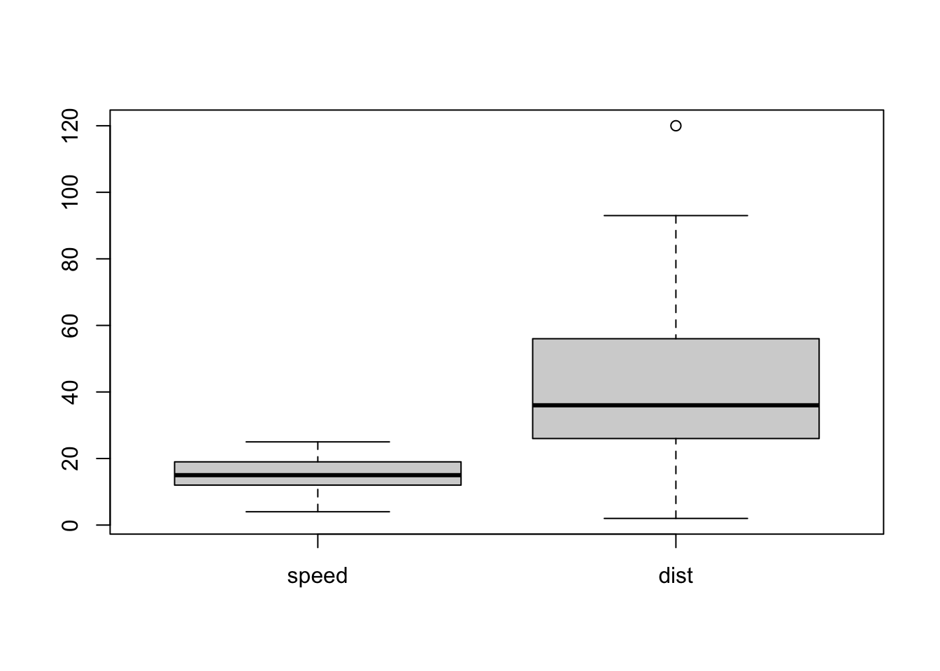
summary(cars)
##      speed           dist       
##  Min.   : 4.0   Min.   :  2.00  
##  1st Qu.:12.0   1st Qu.: 26.00  
##  Median :15.0   Median : 36.00  
##  Mean   :15.4   Mean   : 42.98  
##  3rd Qu.:19.0   3rd Qu.: 56.00  
##  Max.   :25.0   Max.   :120.00
x <- cars$speed
y <- cars$dist

min(x)
## [1] 4
mean(x)
## [1] 15.4
quantile(x)
##   0%  25%  50%  75% 100% 
##    4   12   15   19   25
plot(cars)

abline(lm(cars$dist ~ cars$speed))
summary(lm(cars$dist ~ cars$speed))
## 
## Call:
## lm(formula = cars$dist ~ cars$speed)
## 
## Residuals:
##     Min      1Q  Median      3Q     Max 
## -29.069  -9.525  -2.272   9.215  43.201 
## 
## Coefficients:
##             Estimate Std. Error t value Pr(>|t|)    
## (Intercept) -17.5791     6.7584  -2.601   0.0123 *  
## cars$speed    3.9324     0.4155   9.464 1.49e-12 ***
## ---
## Signif. codes:  0 '***' 0.001 '**' 0.01 '*' 0.05 '.' 0.1 ' ' 1
## 
## Residual standard error: 15.38 on 48 degrees of freedom
## Multiple R-squared:  0.6511, Adjusted R-squared:  0.6438 
## F-statistic: 89.57 on 1 and 48 DF,  p-value: 1.49e-12
boxplot(cars)

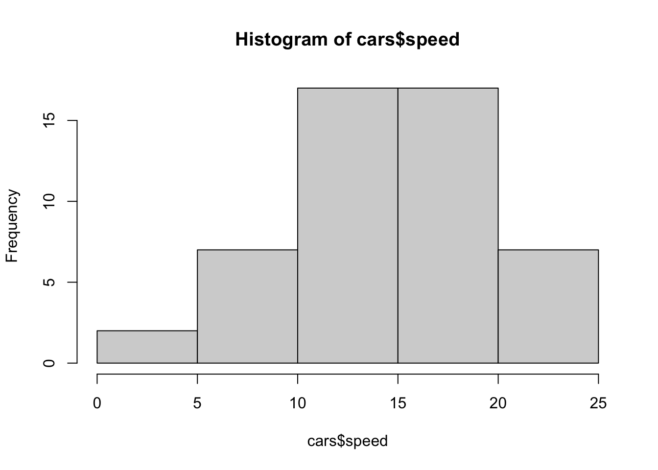
hist(cars$speed)

hist(cars$dist)
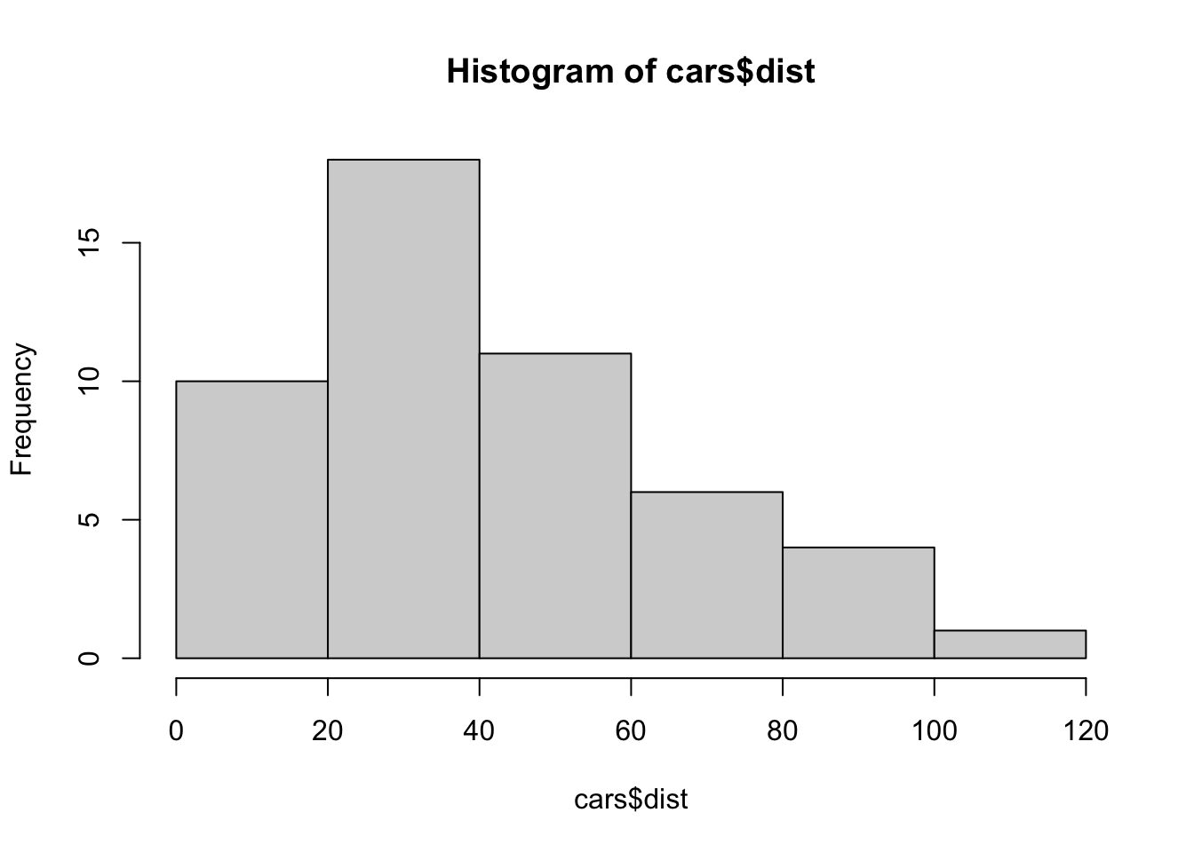
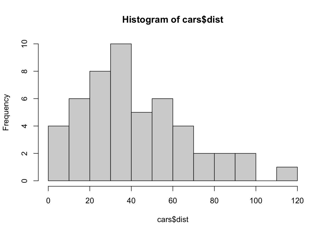
hist(cars$dist, breaks = seq(0,120, 10))
2.1.13.3 Basic Reference

An Introduction to R

2.2 Practicum: Swirl and more on R Script

2.2.1 Swirl: An interactive learning environment for R and statistics

2.2.1.1 Swirl Courses

  1. R Programming: The basics of programming in R
  2. Regression Models: The basics of regression modeling in R
  3. Statistical Inference: The basics of statistical inference in R
  4. Exploratory Data Analysis: The basics of exploring data in R

You can install other swirl courses as well

2.2.2 Install and Start Swirl Courses

2.2.2.1 Three Steps to Start Swirl

install.packages("swirl") # Only the first time.
library(swirl) # Everytime you start swirl
swirl() # Everytime you start or resume swirl

2.2.2.2 R Programming: The basics of programming in R

 1: Basic Building Blocks      2: Workspace and Files     3: Sequences of Numbers    
 4: Vectors                    5: Missing Values          6: Subsetting Vectors      
 7: Matrices and Data Frames   8: Logic                   9: Functions               
10: lapply and sapply         11: vapply and tapply      12: Looking at Data         
13: Simulation                14: Dates and Times        15: Base Graphics          

2.2.2.4 Controling a swirl Session

  • … <– That’s your cue to press Enter to continue

  • You can exit swirl and return to the R prompt (>) at any time by pressing the Esc key.

  • If you are already at the prompt, type bye() to exit and save your progress. When you exit properly, you’ll see a short message letting you know you’ve done so.

When you are at the R prompt (>):

  1. Typing skip() allows you to skip the current question.
  2. Typing play() lets you experiment with R on your own; swirl will ignore what you do…
  3. UNTIL you type nxt() which will regain swirl’s attention.
  4. Typing bye() causes swirl to exit. Your progress will be saved.
  5. Typing main() returns you to swirl’s main menu.
  6. Typing info() displays these options again.
2.2.3 The First EDA using coronavirus.R

  • Pre-installed datasets
  • R Script
    • To access shortcuts, type Option + Shift + K on a Mac, or Alt + Shift + K on Linux and Windows.

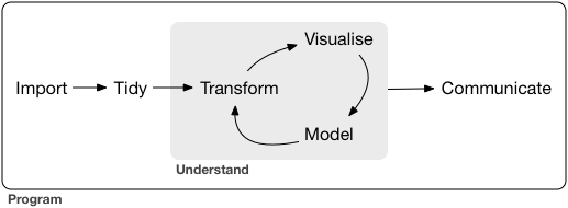
EDA (A diagram from R4DS by H.W. and G.G.)

2.2.4 Basics of Fundamentals of Statistics

2.2.5 Summary

2.2.5.1 Please check the following

  • Installation of R
  • Installation of R Studio
  • Login to RStudio.cloud
  • swirl: R Programming
    • Try 1, 3, 4, 5, 6, 7, 12, 15
  • R Script
    • basics.R - try similar commands
    • coronavirus.R - try different Regions and Periods

2.2.5.2 coronavirus.R

The script and its outputs. coronavirus.csv is too large

# https://coronavirus.jhu.edu/map.html
# JHU Covid-19 global time series data
# See R pakage coronavirus at: https://github.com/RamiKrispin/coronavirus
# Data taken from: https://github.com/RamiKrispin/coronavirus/tree/master/csv
# Last Updated
Sys.Date()
## [1] "2022-11-30"
## Download and read csv (comma separated value) file
coronavirus <- read.csv("https://github.com/RamiKrispin/coronavirus/raw/master/csv/coronavirus.csv")
# write.csv(coronavirus, "data/coronavirus.csv")

## Summaries and structures of the data
head(coronavirus)
##         date province country     lat      long      type cases   uid iso2 iso3
## 1 2020-01-22  Alberta  Canada 53.9333 -116.5765 confirmed     0 12401   CA  CAN
## 2 2020-01-23  Alberta  Canada 53.9333 -116.5765 confirmed     0 12401   CA  CAN
## 3 2020-01-24  Alberta  Canada 53.9333 -116.5765 confirmed     0 12401   CA  CAN
## 4 2020-01-25  Alberta  Canada 53.9333 -116.5765 confirmed     0 12401   CA  CAN
## 5 2020-01-26  Alberta  Canada 53.9333 -116.5765 confirmed     0 12401   CA  CAN
## 6 2020-01-27  Alberta  Canada 53.9333 -116.5765 confirmed     0 12401   CA  CAN
##   code3    combined_key population continent_name continent_code
## 1   124 Alberta, Canada    4413146  North America           <NA>
## 2   124 Alberta, Canada    4413146  North America           <NA>
## 3   124 Alberta, Canada    4413146  North America           <NA>
## 4   124 Alberta, Canada    4413146  North America           <NA>
## 5   124 Alberta, Canada    4413146  North America           <NA>
## 6   124 Alberta, Canada    4413146  North America           <NA>
str(coronavirus)
## 'data.frame':    888636 obs. of  15 variables:
##  $ date          : chr  "2020-01-22" "2020-01-23" "2020-01-24" "2020-01-25" ...
##  $ province      : chr  "Alberta" "Alberta" "Alberta" "Alberta" ...
##  $ country       : chr  "Canada" "Canada" "Canada" "Canada" ...
##  $ lat           : num  53.9 53.9 53.9 53.9 53.9 ...
##  $ long          : num  -117 -117 -117 -117 -117 ...
##  $ type          : chr  "confirmed" "confirmed" "confirmed" "confirmed" ...
##  $ cases         : int  0 0 0 0 0 0 0 0 0 0 ...
##  $ uid           : int  12401 12401 12401 12401 12401 12401 12401 12401 12401 12401 ...
##  $ iso2          : chr  "CA" "CA" "CA" "CA" ...
##  $ iso3          : chr  "CAN" "CAN" "CAN" "CAN" ...
##  $ code3         : int  124 124 124 124 124 124 124 124 124 124 ...
##  $ combined_key  : chr  "Alberta, Canada" "Alberta, Canada" "Alberta, Canada" "Alberta, Canada" ...
##  $ population    : num  4413146 4413146 4413146 4413146 4413146 ...
##  $ continent_name: chr  "North America" "North America" "North America" "North America" ...
##  $ continent_code: chr  NA NA NA NA ...
coronavirus$date <- as.Date(coronavirus$date)
str(coronavirus)
## 'data.frame':    888636 obs. of  15 variables:
##  $ date          : Date, format: "2020-01-22" "2020-01-23" ...
##  $ province      : chr  "Alberta" "Alberta" "Alberta" "Alberta" ...
##  $ country       : chr  "Canada" "Canada" "Canada" "Canada" ...
##  $ lat           : num  53.9 53.9 53.9 53.9 53.9 ...
##  $ long          : num  -117 -117 -117 -117 -117 ...
##  $ type          : chr  "confirmed" "confirmed" "confirmed" "confirmed" ...
##  $ cases         : int  0 0 0 0 0 0 0 0 0 0 ...
##  $ uid           : int  12401 12401 12401 12401 12401 12401 12401 12401 12401 12401 ...
##  $ iso2          : chr  "CA" "CA" "CA" "CA" ...
##  $ iso3          : chr  "CAN" "CAN" "CAN" "CAN" ...
##  $ code3         : int  124 124 124 124 124 124 124 124 124 124 ...
##  $ combined_key  : chr  "Alberta, Canada" "Alberta, Canada" "Alberta, Canada" "Alberta, Canada" ...
##  $ population    : num  4413146 4413146 4413146 4413146 4413146 ...
##  $ continent_name: chr  "North America" "North America" "North America" "North America" ...
##  $ continent_code: chr  NA NA NA NA ...
range(coronavirus$date)
## [1] "2020-01-22" "2022-11-29"
unique(coronavirus$country)
##   [1] "Canada"                           "United Kingdom"                  
##   [3] "China"                            "Netherlands"                     
##   [5] "Australia"                        "New Zealand"                     
##   [7] "Denmark"                          "France"                          
##   [9] "Afghanistan"                      "Albania"                         
##  [11] "Algeria"                          "Andorra"                         
##  [13] "Angola"                           "Antarctica"                      
##  [15] "Antigua and Barbuda"              "Argentina"                       
##  [17] "Armenia"                          "Austria"                         
##  [19] "Azerbaijan"                       "Bahamas"                         
##  [21] "Bahrain"                          "Bangladesh"                      
##  [23] "Barbados"                         "Belarus"                         
##  [25] "Belgium"                          "Belize"                          
##  [27] "Benin"                            "Bhutan"                          
##  [29] "Bolivia"                          "Bosnia and Herzegovina"          
##  [31] "Botswana"                         "Brazil"                          
##  [33] "Brunei"                           "Bulgaria"                        
##  [35] "Burkina Faso"                     "Burma"                           
##  [37] "Burundi"                          "Cabo Verde"                      
##  [39] "Cambodia"                         "Cameroon"                        
##  [41] "Central African Republic"         "Chad"                            
##  [43] "Chile"                            "Colombia"                        
##  [45] "Comoros"                          "Congo (Brazzaville)"             
##  [47] "Congo (Kinshasa)"                 "Costa Rica"                      
##  [49] "Cote d'Ivoire"                    "Croatia"                         
##  [51] "Cuba"                             "Cyprus"                          
##  [53] "Czechia"                          "Diamond Princess"                
##  [55] "Djibouti"                         "Dominica"                        
##  [57] "Dominican Republic"               "Ecuador"                         
##  [59] "Egypt"                            "El Salvador"                     
##  [61] "Equatorial Guinea"                "Eritrea"                         
##  [63] "Estonia"                          "Eswatini"                        
##  [65] "Ethiopia"                         "Fiji"                            
##  [67] "Finland"                          "Gabon"                           
##  [69] "Gambia"                           "Georgia"                         
##  [71] "Germany"                          "Ghana"                           
##  [73] "Greece"                           "Grenada"                         
##  [75] "Guatemala"                        "Guinea"                          
##  [77] "Guinea-Bissau"                    "Guyana"                          
##  [79] "Haiti"                            "Holy See"                        
##  [81] "Honduras"                         "Hungary"                         
##  [83] "Iceland"                          "India"                           
##  [85] "Indonesia"                        "Iran"                            
##  [87] "Iraq"                             "Ireland"                         
##  [89] "Israel"                           "Italy"                           
##  [91] "Jamaica"                          "Japan"                           
##  [93] "Jordan"                           "Kazakhstan"                      
##  [95] "Kenya"                            "Kiribati"                        
##  [97] "Korea, North"                     "Korea, South"                    
##  [99] "Kosovo"                           "Kuwait"                          
## [101] "Kyrgyzstan"                       "Laos"                            
## [103] "Latvia"                           "Lebanon"                         
## [105] "Lesotho"                          "Liberia"                         
## [107] "Libya"                            "Liechtenstein"                   
## [109] "Lithuania"                        "Luxembourg"                      
## [111] "Madagascar"                       "Malawi"                          
## [113] "Malaysia"                         "Maldives"                        
## [115] "Mali"                             "Malta"                           
## [117] "Marshall Islands"                 "Mauritania"                      
## [119] "Mauritius"                        "Mexico"                          
## [121] "Micronesia"                       "Moldova"                         
## [123] "Monaco"                           "Mongolia"                        
## [125] "Montenegro"                       "Morocco"                         
## [127] "Mozambique"                       "MS Zaandam"                      
## [129] "Namibia"                          "Nauru"                           
## [131] "Nepal"                            "Nicaragua"                       
## [133] "Niger"                            "Nigeria"                         
## [135] "North Macedonia"                  "Norway"                          
## [137] "Oman"                             "Pakistan"                        
## [139] "Palau"                            "Panama"                          
## [141] "Papua New Guinea"                 "Paraguay"                        
## [143] "Peru"                             "Philippines"                     
## [145] "Poland"                           "Portugal"                        
## [147] "Qatar"                            "Romania"                         
## [149] "Russia"                           "Rwanda"                          
## [151] "Saint Kitts and Nevis"            "Saint Lucia"                     
## [153] "Saint Vincent and the Grenadines" "Samoa"                           
## [155] "San Marino"                       "Sao Tome and Principe"           
## [157] "Saudi Arabia"                     "Senegal"                         
## [159] "Serbia"                           "Seychelles"                      
## [161] "Sierra Leone"                     "Singapore"                       
## [163] "Slovakia"                         "Slovenia"                        
## [165] "Solomon Islands"                  "Somalia"                         
## [167] "South Africa"                     "South Sudan"                     
## [169] "Spain"                            "Sri Lanka"                       
## [171] "Sudan"                            "Summer Olympics 2020"            
## [173] "Suriname"                         "Sweden"                          
## [175] "Switzerland"                      "Syria"                           
## [177] "Taiwan*"                          "Tajikistan"                      
## [179] "Tanzania"                         "Thailand"                        
## [181] "Timor-Leste"                      "Togo"                            
## [183] "Tonga"                            "Trinidad and Tobago"             
## [185] "Tunisia"                          "Turkey"                          
## [187] "Tuvalu"                           "Uganda"                          
## [189] "Ukraine"                          "United Arab Emirates"            
## [191] "Uruguay"                          "US"                              
## [193] "Uzbekistan"                       "Vanuatu"                         
## [195] "Venezuela"                        "Vietnam"                         
## [197] "West Bank and Gaza"               "Winter Olympics 2022"            
## [199] "Yemen"                            "Zambia"                          
## [201] "Zimbabwe"
unique(coronavirus$type)
## [1] "confirmed" "death"     "recovery"
## Set Country
COUNTRY <- "Japan"
df0 <- coronavirus[coronavirus$country == COUNTRY,]
head(df0)
##              date province country      lat     long      type cases uid iso2
## 183569 2020-01-22     <NA>   Japan 36.20482 138.2529 confirmed     2 392   JP
## 183570 2020-01-23     <NA>   Japan 36.20482 138.2529 confirmed     0 392   JP
## 183571 2020-01-24     <NA>   Japan 36.20482 138.2529 confirmed     0 392   JP
## 183572 2020-01-25     <NA>   Japan 36.20482 138.2529 confirmed     0 392   JP
## 183573 2020-01-26     <NA>   Japan 36.20482 138.2529 confirmed     2 392   JP
## 183574 2020-01-27     <NA>   Japan 36.20482 138.2529 confirmed     0 392   JP
##        iso3 code3 combined_key population continent_name continent_code
## 183569  JPN   392        Japan  126476458           Asia             AS
## 183570  JPN   392        Japan  126476458           Asia             AS
## 183571  JPN   392        Japan  126476458           Asia             AS
## 183572  JPN   392        Japan  126476458           Asia             AS
## 183573  JPN   392        Japan  126476458           Asia             AS
## 183574  JPN   392        Japan  126476458           Asia             AS
tail(df0)
##              date province country      lat     long     type cases uid iso2
## 771815 2022-11-24     <NA>   Japan 36.20482 138.2529 recovery     0 392   JP
## 771816 2022-11-25     <NA>   Japan 36.20482 138.2529 recovery     0 392   JP
## 771817 2022-11-26     <NA>   Japan 36.20482 138.2529 recovery     0 392   JP
## 771818 2022-11-27     <NA>   Japan 36.20482 138.2529 recovery     0 392   JP
## 771819 2022-11-28     <NA>   Japan 36.20482 138.2529 recovery     0 392   JP
## 771820 2022-11-29     <NA>   Japan 36.20482 138.2529 recovery     0 392   JP
##        iso3 code3 combined_key population continent_name continent_code
## 771815  JPN   392        Japan  126476458           Asia             AS
## 771816  JPN   392        Japan  126476458           Asia             AS
## 771817  JPN   392        Japan  126476458           Asia             AS
## 771818  JPN   392        Japan  126476458           Asia             AS
## 771819  JPN   392        Japan  126476458           Asia             AS
## 771820  JPN   392        Japan  126476458           Asia             AS
(pop <- df0$population[1])
## [1] 126476458
df <- df0[c(1,6,7,13)]
str(df)
## 'data.frame':    3129 obs. of  4 variables:
##  $ date      : Date, format: "2020-01-22" "2020-01-23" ...
##  $ type      : chr  "confirmed" "confirmed" "confirmed" "confirmed" ...
##  $ cases     : int  2 0 0 0 2 0 3 0 4 4 ...
##  $ population: num  1.26e+08 1.26e+08 1.26e+08 1.26e+08 1.26e+08 ...
head(df)
##              date      type cases population
## 183569 2020-01-22 confirmed     2  126476458
## 183570 2020-01-23 confirmed     0  126476458
## 183571 2020-01-24 confirmed     0  126476458
## 183572 2020-01-25 confirmed     0  126476458
## 183573 2020-01-26 confirmed     2  126476458
## 183574 2020-01-27 confirmed     0  126476458
### alternatively,
head(df0[c("date", "type", "cases", "population")])
##              date      type cases population
## 183569 2020-01-22 confirmed     2  126476458
## 183570 2020-01-23 confirmed     0  126476458
## 183571 2020-01-24 confirmed     0  126476458
## 183572 2020-01-25 confirmed     0  126476458
## 183573 2020-01-26 confirmed     2  126476458
## 183574 2020-01-27 confirmed     0  126476458
###

## Set types
df_confirmed <- df[df$type == "confirmed",]
df_death <- df[df$type == "death",]
df_recovery <- df[df$data_type == "recovery",]
head(df_confirmed)
##              date      type cases population
## 183569 2020-01-22 confirmed     2  126476458
## 183570 2020-01-23 confirmed     0  126476458
## 183571 2020-01-24 confirmed     0  126476458
## 183572 2020-01-25 confirmed     0  126476458
## 183573 2020-01-26 confirmed     2  126476458
## 183574 2020-01-27 confirmed     0  126476458
head(df_death)
##              date  type cases population
## 484996 2020-01-22 death     0  126476458
## 484997 2020-01-23 death     0  126476458
## 484998 2020-01-24 death     0  126476458
## 484999 2020-01-25 death     0  126476458
## 485000 2020-01-26 death     0  126476458
## 485001 2020-01-27 death     0  126476458
head(df_recovery)
## [1] date       type       cases      population
##  <0 行> (または長さ 0 の row.names)
## Histogram
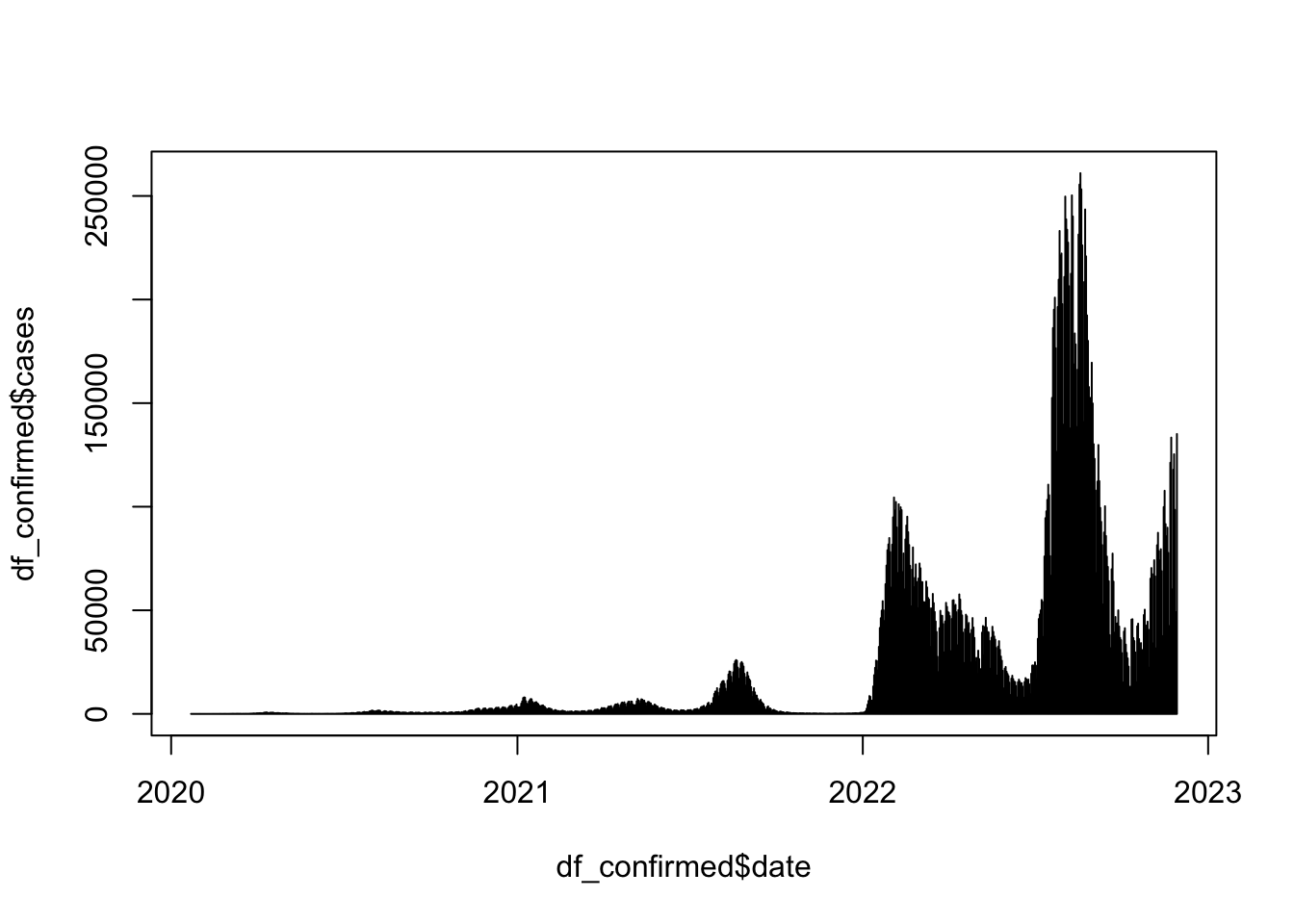
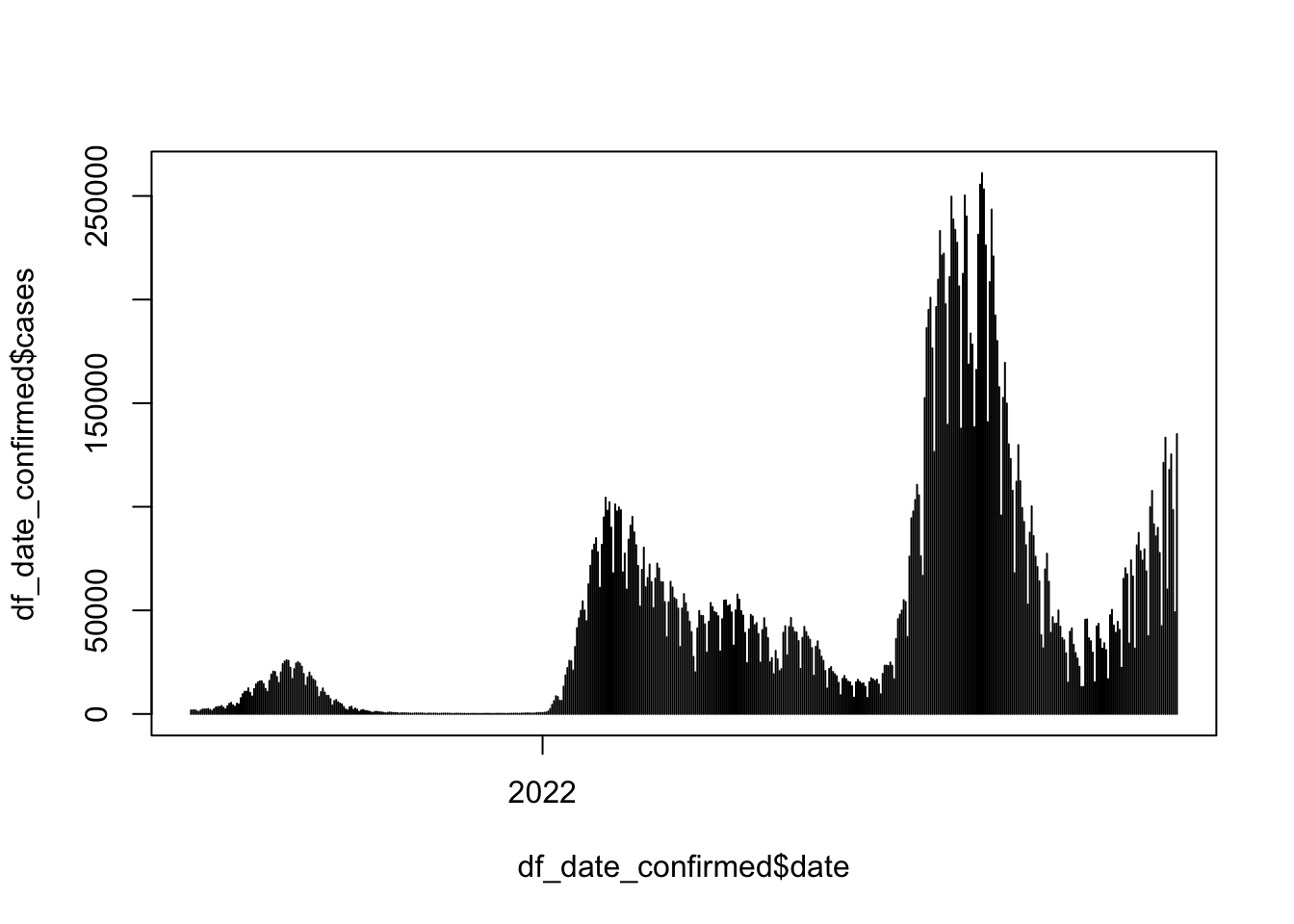
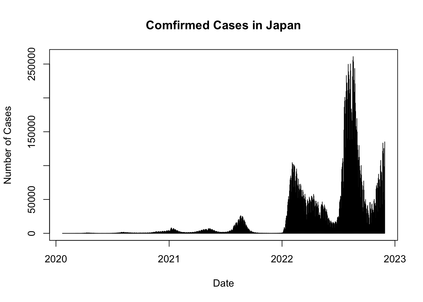
plot(df_confirmed$date, df_confirmed$cases, type = "h")

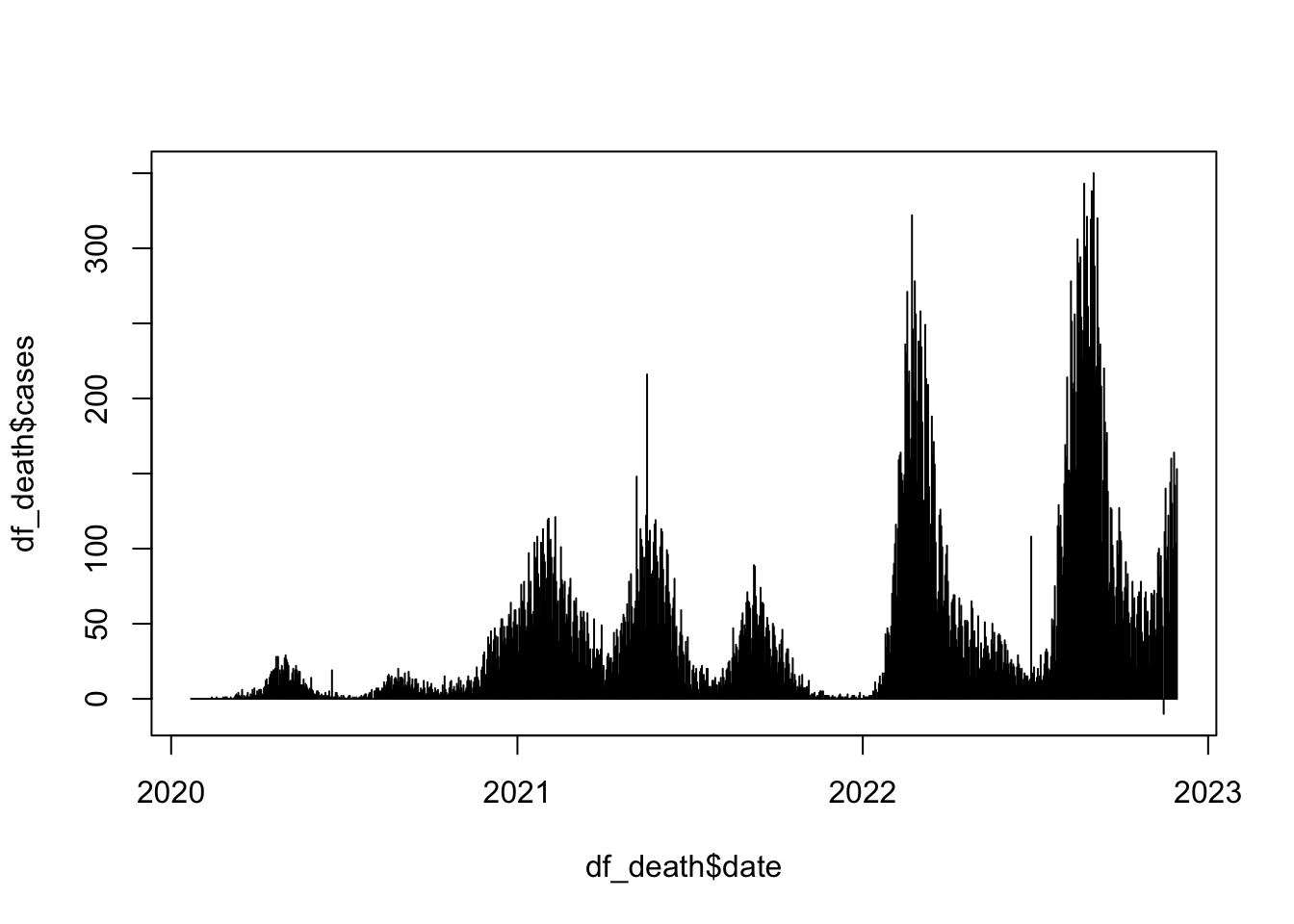
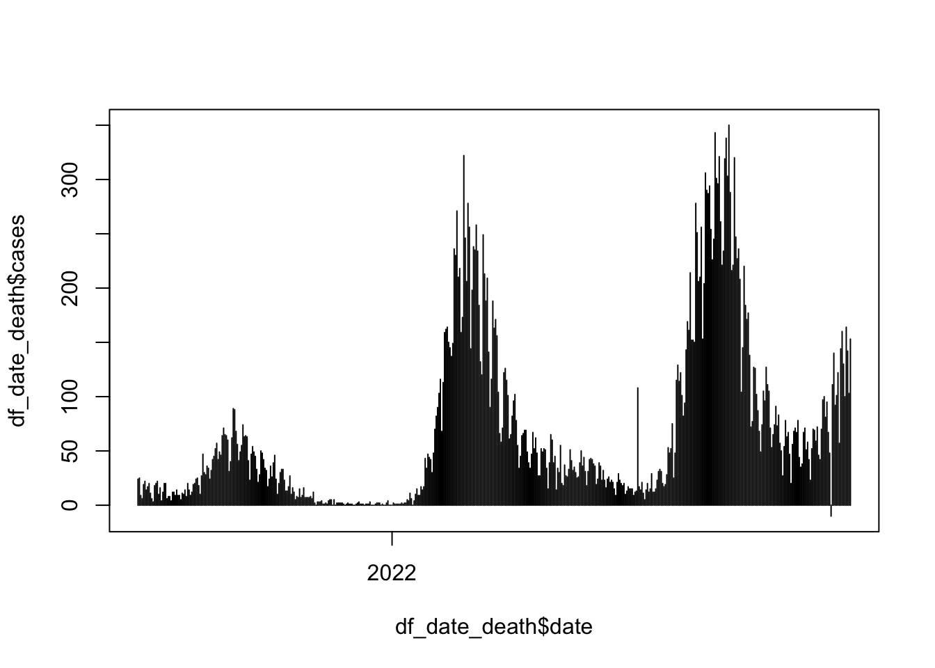
plot(df_death$date, df_death$cases, type = "h")

# plot(df_recovered$date, df_recovered$cases, type = "h") # no data for recovery

## Scatter plot and correlation
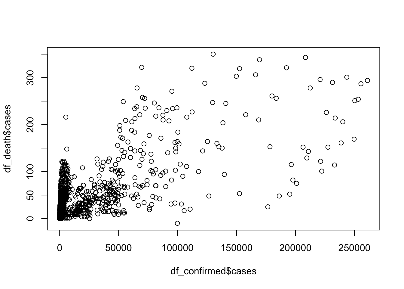
plot(df_confirmed$cases, df_death$cases, type = "p")

cor(df_confirmed$cases, df_death$cases)
## [1] 0.716229
## In addition set a period
start_date <- as.Date("2021-07-01")
end_date <- Sys.Date() 
df_date <- df[df$date >=start_date & df$date <= end_date,]
##

## Set types
df_date_confirmed <- df_date[df_date$type == "confirmed",]
df_date_death <- df_date[df_date$type == "death",]
df_date_recovery <- df_date[df_date$data_type == "recovery",]
head(df_date_confirmed)
##              date      type cases population
## 184095 2021-07-01 confirmed  1754  126476458
## 184096 2021-07-02 confirmed  1775  126476458
## 184097 2021-07-03 confirmed  1878  126476458
## 184098 2021-07-04 confirmed  1485  126476458
## 184099 2021-07-05 confirmed  1029  126476458
## 184100 2021-07-06 confirmed  1668  126476458
head(df_date_death)
##              date  type cases population
## 485522 2021-07-01 death    24  126476458
## 485523 2021-07-02 death    25  126476458
## 485524 2021-07-03 death     9  126476458
## 485525 2021-07-04 death     6  126476458
## 485526 2021-07-05 death    19  126476458
## 485527 2021-07-06 death    22  126476458
head(df_date_recovery)
## [1] date       type       cases      population
##  <0 行> (または長さ 0 の row.names)
## Histogram
plot(df_date_confirmed$date, df_date_confirmed$cases, type = "h")

plot(df_date_death$date, df_date_death$cases, type = "h")

# plot(df_date_recovered$date, df_date_recovered$cases, type = "h") # no data for recovery

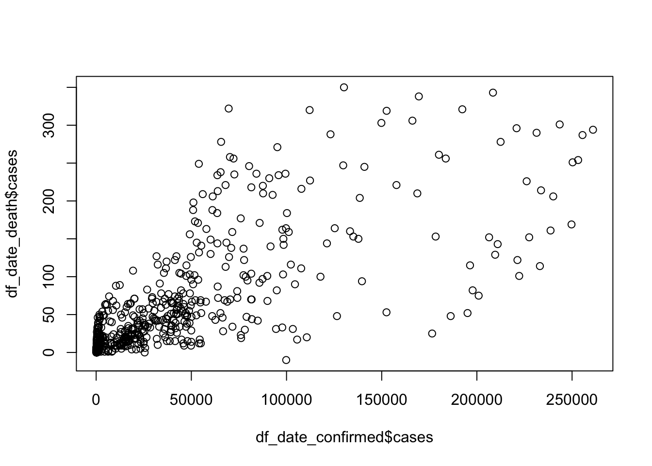
plot(df_date_confirmed$cases, df_date_death$cases, type = "p")

cor(df_date_confirmed$cases, df_date_death$cases)
## [1] 0.7289401
### Q0. Change the values of the location and the period and see the outcomes.
### Q1. What is the correlation between df_confirmed$cases and df_death$cases?
### Q2. Do we have a larger correlation value if we shift the dates to implement the time-lag?
### Q3. Do you have any other questions to explore?

#### Extra
plot(df_confirmed$date, df_confirmed$cases, type = "h", 
     main = paste("Comfirmed Cases in",COUNTRY), 
     xlab = "Date", ylab = "Number of Cases")

2.2.5.3 Assignment 1 and Assignment 2: Questions and a Quiz in Moodle

Please complete assignments in Moodle by 2021-12-21