Chapter 5 Exploratory Data Analysis (EDA) 4

Course Contents

1. 2021-12-08: Introduction: About the course
   - An introduction to open and public data, and data science
2. 2021-12-15: Exploratory Data Analysis (EDA) 1 [lead by hs]
   - R Basics with RStudio and/or RStudio.cloud; R Script, swirl
3. 2021-12-22: Exploratory Data Analysis (EDA) 2 [lead by hs]
   - R Markdown; Introduction to tidyverse; RStudio Primers
4. 2022-01-12: Exploratory Data Analysis (EDA) 3 [lead by hs]
   - Introduction to tidyverse; Public Data, WDI, etc
5. 2022-01-19: Exploratory Data Analysis (EDA) 4 [lead by hs]
   - Introduction to tidyverse; WDI, UN, , etc
6. 2022-01-26: Exploratory Data Analysis (EDA) 5 [lead by hs]
   - Introduction to tidyverse; WDI, WHO, OECD, US gov, etc
7. 2022-02-02: Inference Statistics 1
8. 2022-02-09: Inference Statistics 2
9. 2022-02-16: Inference Statistics 3
10. 2022-02-23: Project Presentation

Transforming and Tidying Data

• Transforming Data by dplyr for EDA
• Tidying Data by tidyr

EDA (A diagram from R4DS by H.W. and G.G.)

EDA from r4ds

Contents of EDA4

• More on Transforming Data by dplyr

  • select, filter, mutate, arrange, group_by, summarize, etc.

• Tidying Data by tidyr

  • pivot_longer, pivot_wider, drop_na, etc

• Example: A Study of Cases of Coronavirus Pandemic, III

• Importing Various Public Data and Examples
  • WDI, World Bank, read_xl, i.e., read_excel, etc., for WDI Class Data
  • UN data
  • etc.

5.1 Part I: More on Transforming by dplyr and Tidying by tidyr

5.1.1 Data Transforamtion by dplyr Overview – r4ds.

dplyr is a grammar of data manipulation, providing a consistent set of verbs that help you solve the most common data manipulation challenges:

• select() picks variables based on their names.
• filter() picks cases based on their values.
• mutate() adds new variables that are functions of existing variables
• arrange() changes the ordering of the rows.
• summarise() reduces multiple values down to a single summary.
  • summarise() and summarize() are synonyms.
• group_by() converts into a grouped tbl where operations are performed “by group”. ungroup() removes grouping.
• slice() lets you index rows by their (integer) locations. It allows you to select, remove, and duplicate rows.

5.1.2 select: Subset columns using their names and types

Helper	Use	Example
-	Columns except	select(babynames, -prop)
:	Columns between	select(babynames, year:n)
contains()	Columns that contains a string	select(babynames, contains(“n”))
ends_with()	Columns that ends with a string	select(babynames, ends_with(“n”))
matches()	Columns that matches a regex	select(babynames, matches(“n”))
num_range()	Columns with a numerical suffix in the range	Not applicable with babynames
one_of()	Columns whose name appear in the given set	select(babynames, one_of(c(“sex”, “gender”)))
starts_with()	Columns that starts with a string	select(babynames, starts_with(“n”))

5.1.3 iris

##   Sepal.Length Sepal.Width Petal.Length Petal.Width Species
## 1          5.1         3.5          1.4         0.2  setosa
## 2          4.9         3.0          1.4         0.2  setosa
## 3          4.7         3.2          1.3         0.2  setosa
## 4          4.6         3.1          1.5         0.2  setosa
## 5          5.0         3.6          1.4         0.2  setosa
## 6          5.4         3.9          1.7         0.4  setosa

colnames(iris) <- c("Sepal.L", "Sepal.W", "Petal.L", "Petal.W", "Species")

slice(iris, 1:10)

##    Sepal.L Sepal.W Petal.L Petal.W Species
## 1      5.1     3.5     1.4     0.2  setosa
## 2      4.9     3.0     1.4     0.2  setosa
## 3      4.7     3.2     1.3     0.2  setosa
## 4      4.6     3.1     1.5     0.2  setosa
## 5      5.0     3.6     1.4     0.2  setosa
## 6      5.4     3.9     1.7     0.4  setosa
## 7      4.6     3.4     1.4     0.3  setosa
## 8      5.0     3.4     1.5     0.2  setosa
## 9      4.4     2.9     1.4     0.2  setosa
## 10     4.9     3.1     1.5     0.1  setosa

5.1.4 select: Example

slice(select(iris, sl = Sepal.L, sw = Sepal.W, 
             species = Species), 1:2)

##    sl  sw species
## 1 5.1 3.5  setosa
## 2 4.9 3.0  setosa

slice(select(iris, Petal.L:Species),1:2)

##   Petal.L Petal.W Species
## 1     1.4     0.2  setosa
## 2     1.4     0.2  setosa

5.1.5 filter: Subset rows using column values

Logical operator	tests	Example
>	Is x greater than y?	x > y
>=	Is x greater than or equal to y?	x >= y
<	Is x less than y?	x < y
<=	Is x less than or equal to y?	x <= y
==	Is x equal to y?	x == y
!=	Is x not equal to y?	x != y
is.na()	Is x an NA?	is.na(x)
!is.na()	Is x not an NA?	!is.na(x)

filter(iris, (Species == "versicolor") & 
         Sepal.L %in% c(6.7, 7.0))

##   Sepal.L Sepal.W Petal.L Petal.W    Species
## 1     7.0     3.2     4.7     1.4 versicolor
## 2     6.7     3.1     4.4     1.4 versicolor
## 3     6.7     3.0     5.0     1.7 versicolor
## 4     6.7     3.1     4.7     1.5 versicolor

filter(iris, (Species == "versicolor") & 
         (Sepal.L >= 6.7 & Sepal.L <= 7.0))

##   Sepal.L Sepal.W Petal.L Petal.W    Species
## 1     7.0     3.2     4.7     1.4 versicolor
## 2     6.9     3.1     4.9     1.5 versicolor
## 3     6.7     3.1     4.4     1.4 versicolor
## 4     6.8     2.8     4.8     1.4 versicolor
## 5     6.7     3.0     5.0     1.7 versicolor
## 6     6.7     3.1     4.7     1.5 versicolor

5.1.6 mutate

• Create, modify, and delete columns

• Useful mutate functions

  • +, -, log(), etc., for their usual mathematical meanings

  • lead(), lag()

  • dense_rank(), min_rank(), percent_rank(), row_number(), cume_dist(), ntile()

  • cumsum(), cummean(), cummin(), cummax(), cumany(), cumall()

  • na_if(), coalesce()

  • if_else(), recode(), case_when()

5.1.7 arrange and Pipe %>%

• arrange() orders the rows of a data frame by the values of selected columns.

Unlike other dplyr verbs, arrange() largely ignores grouping; you need to explicitly mention grouping variables (`or use .by_group = TRUE) in order to group by them, and functions of variables are evaluated once per data frame, not once per group.

• pipes in R for Data Science.

Examples

arrange(<data>, <varible>)
arrange(<data>, desc(<variable>))

<data> %>% ggplot() + geom_point(aes(x = <>, y = <>))

5.1.8 group_by() and summarise()

• group_by
• summarise or summarize

iris %>% 
  group_by(Species) %>% 
  summarize(sl = mean(Sepal.L), sw = mean(Sepal.W), 
  pl = mean(Petal.L), pw = mean(Petal.W))

## # A tibble: 3 × 5
##   Species       sl    sw    pl    pw
##   <fct>      <dbl> <dbl> <dbl> <dbl>
## 1 setosa      5.01  3.43  1.46 0.246
## 2 versicolor  5.94  2.77  4.26 1.33 
## 3 virginica   6.59  2.97  5.55 2.03

5.1.9 Tidy Data

“Happy families are all alike; every unhappy family is unhappy in its own way.” Leo Tolstoy

“Tidy datasets are all alike, but every messy dataset is messy in its own way.” Hadley Wickham

5.1.9.1 Three interrelated rules of a tidy dataset

1. Each variable must have its own column.
2. Each observation must have its own row.
3. Each value must have its own cell.

5.1.10 Tidy Data and Untidy Data, I

The following examples are taken from r4ds, 12. Tidy data.

table1

## # A tibble: 6 × 4
##   country      year  cases population
##   <chr>       <int>  <int>      <int>
## 1 Afghanistan  1999    745   19987071
## 2 Afghanistan  2000   2666   20595360
## 3 Brazil       1999  37737  172006362
## 4 Brazil       2000  80488  174504898
## 5 China        1999 212258 1272915272
## 6 China        2000 213766 1280428583

5.1.11 Tidy Data and Untidy Data, II

table2

## # A tibble: 12 × 4
##    country      year type            count
##    <chr>       <int> <chr>           <int>
##  1 Afghanistan  1999 cases             745
##  2 Afghanistan  1999 population   19987071
##  3 Afghanistan  2000 cases            2666
##  4 Afghanistan  2000 population   20595360
##  5 Brazil       1999 cases           37737
##  6 Brazil       1999 population  172006362
##  7 Brazil       2000 cases           80488
##  8 Brazil       2000 population  174504898
##  9 China        1999 cases          212258
## 10 China        1999 population 1272915272
## 11 China        2000 cases          213766
## 12 China        2000 population 1280428583

5.1.12 Tidy Data and Untidy Data, III

table3

## # A tibble: 6 × 3
##   country      year rate             
## * <chr>       <int> <chr>            
## 1 Afghanistan  1999 745/19987071     
## 2 Afghanistan  2000 2666/20595360    
## 3 Brazil       1999 37737/172006362  
## 4 Brazil       2000 80488/174504898  
## 5 China        1999 212258/1272915272
## 6 China        2000 213766/1280428583

5.1.13 Tidy Data and Untidy Data, IV

table4a; table4b

## # A tibble: 3 × 3
##   country     `1999` `2000`
## * <chr>        <int>  <int>
## 1 Afghanistan    745   2666
## 2 Brazil       37737  80488
## 3 China       212258 213766

## # A tibble: 3 × 3
##   country         `1999`     `2000`
## * <chr>            <int>      <int>
## 1 Afghanistan   19987071   20595360
## 2 Brazil       172006362  174504898
## 3 China       1272915272 1280428583

5.1.14 Tidy Data and Untidy Data, V

table5

## # A tibble: 6 × 4
##   country     century year  rate             
## * <chr>       <chr>   <chr> <chr>            
## 1 Afghanistan 19      99    745/19987071     
## 2 Afghanistan 20      00    2666/20595360    
## 3 Brazil      19      99    37737/172006362  
## 4 Brazil      20      00    80488/174504898  
## 5 China       19      99    212258/1272915272
## 6 China       20      00    213766/1280428583

5.1.15 Tidying Data with pivot_longer, and pivot_wider

5.1.15.1 tidyr: Pivoting

• pivot_longer():Pivot data from wide to long, [old: gather()]

pivot_longer(data = <data>, cols = <column>, 
    names_to = <new column>, values_to = <value column>)

pivot_longer(data = table4a, cols = c(1999,2000), 
    names_to = "year", values_to = "population" )

• pivot_wider():Pivot data from long to wide, [old: spread()]

pivot_wider(data = <data>, names_from = <specified column>, 
    values_from = <value column>)

pivot_wider(data = table2, names_from = type, 
    values_from = count)

5.1.16 Example 1: pivot_longer

table4a

## # A tibble: 3 × 3
##   country     `1999` `2000`
## * <chr>        <int>  <int>
## 1 Afghanistan    745   2666
## 2 Brazil       37737  80488
## 3 China       212258 213766

pivot_longer(data = table4a, cols = c("1999","2000"), 
             names_to = "year", values_to = "cases",
             names_transform = list("year" = as.integer))

5.1.17 Example 1: pivot_longer

pivot_longer(data = table4a, cols = c("1999","2000"), 
             names_to = "year", values_to = "cases", 
             names_transform = list("year" = as.integer))

## # A tibble: 6 × 3
##   country      year  cases
##   <chr>       <int>  <int>
## 1 Afghanistan  1999    745
## 2 Afghanistan  2000   2666
## 3 Brazil       1999  37737
## 4 Brazil       2000  80488
## 5 China        1999 212258
## 6 China        2000 213766

5.1.18 Example 2: pivot_wider

table2 %>% slice(1:4)

## # A tibble: 4 × 4
##   country      year type          count
##   <chr>       <int> <chr>         <int>
## 1 Afghanistan  1999 cases           745
## 2 Afghanistan  1999 population 19987071
## 3 Afghanistan  2000 cases          2666
## 4 Afghanistan  2000 population 20595360

pivot_wider(data = table2, names_from = type, 
            values_from = count)

5.1.19 Example 2: pivot_wider

pivot_wider(data = table2, names_from = type, 
            values_from = count)

## # A tibble: 6 × 4
##   country      year  cases population
##   <chr>       <int>  <int>      <int>
## 1 Afghanistan  1999    745   19987071
## 2 Afghanistan  2000   2666   20595360
## 3 Brazil       1999  37737  172006362
## 4 Brazil       2000  80488  174504898
## 5 China        1999 212258 1272915272
## 6 China        2000 213766 1280428583

5.1.20 Example 3: separate

• Separate a character column into multiple columns with a regular expression or numeric locations

table3 %>% slice(1:4)

## # A tibble: 4 × 3
##   country      year rate           
##   <chr>       <int> <chr>          
## 1 Afghanistan  1999 745/19987071   
## 2 Afghanistan  2000 2666/20595360  
## 3 Brazil       1999 37737/172006362
## 4 Brazil       2000 80488/174504898

separate(table3, rate, c("cases", "population"), 
         sep = "/", convert = TRUE)

5.1.21 Example 3: separate

• Separate a character column into multiple columns with a regular expression or numeric locations

separate(table3, rate, c("cases", "population"), 
         sep = "/", convert = TRUE)

## # A tibble: 6 × 4
##   country      year  cases population
##   <chr>       <int>  <int>      <int>
## 1 Afghanistan  1999    745   19987071
## 2 Afghanistan  2000   2666   20595360
## 3 Brazil       1999  37737  172006362
## 4 Brazil       2000  80488  174504898
## 5 China        1999 212258 1272915272
## 6 China        2000 213766 1280428583

5.1.22 Example 3: unite

• Unite multiple columns into one by pasting strings together

table5 %>% slice(1:4)

## # A tibble: 4 × 4
##   country     century year  rate           
##   <chr>       <chr>   <chr> <chr>          
## 1 Afghanistan 19      99    745/19987071   
## 2 Afghanistan 20      00    2666/20595360  
## 3 Brazil      19      99    37737/172006362
## 4 Brazil      20      00    80488/174504898

table5 %>% unite(col = "year", century, year, sep = "") %>%
  separate(rate, c("cases", "population"), sep = "/", 
           convert = TRUE) %>%
  mutate(year = as.integer(year), rate = cases / population)

5.1.23 Example 3: unite

• Unite multiple columns into one by pasting strings together

table5 %>% unite(col = "year", century, year, sep = "") %>%
  separate(rate, c("cases", "population"), sep = "/", 
           convert = TRUE) %>%
  mutate(year = as.integer(year), rate = cases / population)

## # A tibble: 6 × 5
##   country      year  cases population      rate
##   <chr>       <int>  <int>      <int>     <dbl>
## 1 Afghanistan  1999    745   19987071 0.0000373
## 2 Afghanistan  2000   2666   20595360 0.000129 
## 3 Brazil       1999  37737  172006362 0.000219 
## 4 Brazil       2000  80488  174504898 0.000461 
## 5 China        1999 212258 1272915272 0.000167 
## 6 China        2000 213766 1280428583 0.000167

5.1.24 Example 5: bind_rows

table4a; table4b

## # A tibble: 3 × 3
##   country     `1999` `2000`
## * <chr>        <int>  <int>
## 1 Afghanistan    745   2666
## 2 Brazil       37737  80488
## 3 China       212258 213766

## # A tibble: 3 × 3
##   country         `1999`     `2000`
## * <chr>            <int>      <int>
## 1 Afghanistan   19987071   20595360
## 2 Brazil       172006362  174504898
## 3 China       1272915272 1280428583

5.1.25 Example 5: bind_rows - 1st Step

tables <- list(cases = table4a, population = table4b)
tables %>% bind_rows(.id = "type")

## # A tibble: 6 × 4
##   type       country         `1999`     `2000`
##   <chr>      <chr>            <int>      <int>
## 1 cases      Afghanistan        745       2666
## 2 cases      Brazil           37737      80488
## 3 cases      China           212258     213766
## 4 population Afghanistan   19987071   20595360
## 5 population Brazil       172006362  174504898
## 6 population China       1272915272 1280428583

5.1.26 Example 5: bind_rows

tables <- list(cases = table4a, population = table4b)
tables %>% bind_rows(.id = "type") %>%
  pivot_longer(cols = c("1999", "2000"), names_to = "year") %>%
  pivot_wider(names_from = "type", values_from = "value") %>%
  mutate(year = as.integer(year)) %>% arrange(country)

## # A tibble: 6 × 4
##   country      year  cases population
##   <chr>       <int>  <int>      <int>
## 1 Afghanistan  1999    745   19987071
## 2 Afghanistan  2000   2666   20595360
## 3 Brazil       1999  37737  172006362
## 4 Brazil       2000  80488  174504898
## 5 China        1999 212258 1272915272
## 6 China        2000 213766 1280428583

5.1.27 Example I

A Study of Cases of Coronavirus Pandemic, III

5. Data of Johns Hopkins Universiy and World Bank

• 5.1 Importing Raw Data
• 5.2 Tidying and Combining: To create country level and global combined data
• 5.3 Aggregated by Countries
• 5.4 Population of 2019
• 5.5 Analysis Suggested by Rami Krispin

5.2 Part II: Various Databases

5.2.1 Example II

Introduction to Public Data

2. World Bank

• 2.6 World Bank Country and Lending Groups and an Option extra = TRUE
  • 2.6.1 Review Basics: World Development Indicators: ?WDI
  • 2.6.2 World Bank Country and Lending Groups
  • 2.6.3 Importing Excel Files
  • 2.6.4 Filtering Join
  • 2.6.5 Join Tables
  • 2.6.6 Join Tables: Quick References

3. United Nations

• 3.1 Importing Data
• 3.2 Example

5.2.2 World Development Indicators: ?WDI

1. Basic Usage

WDI(country = "all", indicator = "NY.GDP.PCAP.KD")

2. Vector Notation

WDI(country = c("US", "CN", JP"), # ISO-2 codes
   indicator = c("gdp_pcap" = "NY.GDP.PCAP.KD", 
                "life_exp" = "SP.DYN.LE00.IN"))

3. Use Extra

WDI(country = "all", 
   indicator = c("gdp_pcap" = NY.GDP.PCAP.KD", 
                "life_exp" = "SP.DYN.LE00.IN"), extra = TRUE)

extra: TRUE returns extra variables such as region, iso3c code, and incomeLevel

5.2.3 World Bank Country and Lending Groups

• URL World Bank Country and Lending Groups
• The current classification by income in XLS format

5.2.3.1 About CLASS.xlsx

This table classifies all World Bank member countries (189), and all other economies with populations of more than 30,000. For operational and analytical purposes, economies are divided among income groups according to 2019 gross national income (GNI) per capita, calculated using the World Bank Atlas method. The groups are:

• low income, $1,035 or less;
• lower middle income, $1,036 - 4,045;
• upper middle income, $4,046 - 12,535;
• and high income, $12,536 or more.

The effective operational cutoff for IDA eligibility is $1,185 or less.

5.2.3.2 Geographic classifications

• IDA countries are those that lack the financial ability to borrow from IBRD.

• IDA credits are deeply concessional—interest-free loans and grants for programs aimed at boosting economic growth and improving living conditions.

• IBRD loans are noncessional.

• Blend countries are eligible for IDA credits because of their low per capita incomes but are also eligible for IBRD because they are financially creditworthy.

5.2.3.3 Note

• The term country, used interchangeably with economy, does not imply political independence but refers to any territory for which authorities report separate social or economic statistics.

• Income classifications set on 1 July 2020 remain in effect until 1 July 2021.

• Argentina, which was temporarily unclassified in July 2016 pending release of revised national accounts statistics, was classified as upper middle income for FY17 as of 29 September 2016 based on alternative conversion factors. Also effective 29 September 2016, Syrian Arab Republic is reclassified from IBRD lending category to IDA-only.

• On 29 March 2017, new country codes were introduced to align World Bank 3-letter codes with ISO 3-letter codes: Andorra (AND), Dem. Rep. Congo (COD), Isle of Man (IMN), Kosovo (XKX), Romania (ROU), Timor-Leste (TLS), and West Bank and Gaza (PSE).

5.2.4 Importing Excel Files, Part I

• CLASS.xlsx: - copy the following link
  • The current classification by income in XLS format
• readxl: https://readxl.tidyverse.org
• Help: read_excel, read_xls, read_xlsx

url_class <- "http://databank.worldbank.org/ 
  data/download/site-content/CLASS.xlsx"
download.file(url = url_class, destfile = "data/CLASS.xlsx")

library(readxl)
wb_countries_tmp <- read_excel("data/CLASS.xlsx", 
  sheet = 1, skip = 4, n_max =219) %>% slice(-1)
wb_countries <- wb_countries_tmp %>% 
  select(Economy, Code, Region, `Income group`, 
        Code, Region:Other)
wb_countries

5.2.5 Importing Excel Files, Part II

• readxl: https://readxl.tidyverse.org
• Help: read_excel, read_xls, read_xlsx

wb_regions_tmp <- read_excel("data/CLASS.xlsx", 
  sheet = 1, skip = 4, n_max =272) %>% 
  slice(-(1:221))
wb_regions <- wb_regions_tmp %>% 
  select(Economy:Code) %>% drop_na()
wb_regions

wb_groups_tmp <- read_excel("data/CLASS.xlsx", 
  sheet = "Groups") # sheet = 3
wb_groups_tmp

• Please study ‘About Assignment Five’ in Moodle

5.2.6 Filtering Joins

gdp_pcap <- WDI(country = "all", 
    indicator = "NY.GDP.PCAP.KD")
gdp_pcap_extra <- WDI(country = "all", 
    indicator = "NY.GDP.PCAP.KD", extra = TRUE)

• Compare the following:

gdp_pcap %>% semi_join(country_list)

gdp_pcap %>% filter(region != "Aggregates")

gdp_pcap %>% anti_join(country_list)

• Please study ‘About Assignment Five’ in Moodle

5.2.7 Join Tables

There are three types of joining tables. Commands are from tidyverse packages though there is a way to do the same by Base R with appropriate arguments.

1. Bind rows: bind_rows(), intersect(), setdiff(), union()
2. Bind columns: bind_cols(), left_join(), right_join(), inner_join(), full_join()
3. Filtering join: semi_join(), anti_join()

5.2.8 Join Tables: Quick References

1. https://r4ds.had.co.nz/relational-data.html#relational-data

2. Cheatsheet: Data Transformation, pages 2 and 3. You can download it from RStudio > Help.

3. Tidyverse Homepage:

   1. Efficiently bind multiple data frames by row and column: bind_rows(), bind_cols()
   2. Set operations: intersect(), setdiff(), union()
   3. Mutating joins: left_join(), right_join(), inner_join(), full_join()
   4. Filtering joins: semi_join(), anti_join()

4. R Studio Primers: Tidy Your Data – r4ds: Wrangle, II

   • Reshape Data, Separate and Unite Columns, Join Data Sets

5.2.9 Public Data: UN Data

• UN Data: https://data.un.org

5.2.9.1 Importing Data

1. Get the URL (uniform resource locator) - copy the link

• url_of_data <- "https://data.un.org/--long url--.csv"

2. Download the file into the destfile in data folder:

• download.file(url = url_of_data, destfile = "data/un_pop.csv")

3. Read the file:

• df_un_pop <- read_csv("data/un_pop.csv")

5.2.10 Learning Resources, IV

• R for Data Science, Part III Wrangle
• R for Data Science, Part III Wrangle - Tidy and Relational
• Tidy Data: https://vita.had.co.nz/papers/tidy-data.pdf
  • https://github.com/hadley/tidy-data

5.2.10.1 RStudio Primers: See References in Moodle at the bottom

1. The Basics – r4ds: Explore, I
2. Work with Data – r4ds: Wrangle, I
3. Visualize Data – r4ds: Explore, II

• Exploratory Data Analysis, Bar Charts, Histograms
• Boxplots and Counts, Scatterplots, Line Plots
• Overplotting and Big Data, Customize Your Plots

4. Tidy Your Data – r4ds: Wrangle, II

• Reshape Data, Separate and Unite Columns, Join Data Sets

5.2.11 The Fifth Assignment (in Moodle)

• Choose a World Bank or UN data. Clearly state how to obtain the data. Even if you are able to give the URL to download the data, explain the steps you reached and obtained the data.

• If you choose WDI, use CLASS.xlsx, World Bank Country and Lending Groups information.

• Create an R Notebook (file name.nb.html) of an EDA containing:

  1. title, date, and author, i.e., Your Name
  2. your motivation and/or objectives to analyse the data, and your questions
  3. an explanation of the data and the variables
  4. chunks containing the following:
     • visualize the data with ggplot()
  5. your findings and/or questions
  6. file name: a5_ID.nb.html, e.g. a5_123456.nb.html

• Submit your R Notebook file to Moodle (The Fifth Assignment) by 2022-01-25 23:59:00

5.3 Responses to the Fifth Assignment

5.3.1 Setup and YAML

library(tidyverse)
library(WDI)

5.4 CLASS.xlsx

5.4.1 Introduction

There are several reasons we study CLASS.xlsx

WDI data contains not only the data of each country but the aggregated data of regions, income level, etc. We need to know the definitions of these groups and countries in them. CLASS.xlsx provides the information.

Why are groups important? When we study a trend of data of a country, we need to look at the following.

1. The trends of the aggregated data of the World.
2. The comparison of the trends of the aggregated data of groups.
3. The comparison of the trends of the data of the countries within the group the country of your interest belongs to.

We first download CLASS.xlsx from world bank and obtain the data so that we can use it with other data.

See Introduction to Public Data in Moodle, Week 5.

5.4.1.1 Importing Excel Files

• CLASS.xlsx: - copy the following link
  • The current classification by income in XLS format
• readxl: https://readxl.tidyverse.org
• Help: read_excel, read_xls, read_xlsx

url_class <- "https://databankfiles.worldbank.org/data/download/site-content/CLASS.xlsx"
download.file(url = url_class, destfile = "data/CLASS.xlsx")

5.4.1.1.1 Countries

Let us look at the first sheet.

1. The column names are in the 5th row.
2. The country data starts from the 7th row.
3. Zimbabue is at the last row.

library(readxl)
wb_countries_tmp <- read_excel("data/CLASS.xlsx", sheet = 1, skip = 0, n_max =219) 
wb_countries <- wb_countries_tmp %>% 
  select(country = Economy, iso3c = Code, region = Region, income = `Income group`, lending = "Lending category", other = "Other (EMU or HIPC)")
DT::datatable(wb_countries)

5.4.1.1.2 Regions

• readxl: https://readxl.tidyverse.org
• Help: read_excel, read_xls, read_xlsx

1. Regions start from the 221th row.
2. Regions end at the 266th row.

wb_regions_tmp <- read_excel("data/CLASS.xlsx", sheet = 1, skip = 0, n_max =266) %>% 
  slice(-(1:220))
wb_regions <- wb_regions_tmp %>% 
  select(region = Economy, iso3c = Code) %>% drop_na()
DT::datatable(wb_regions)

Let us look at the second sheet.

wb_groups_tmp <- read_excel("data/CLASS.xlsx", sheet = "Groups") # sheet = 3
wb_groups <- wb_groups_tmp %>% 
  select(gcode = GroupCode, group = GroupName, iso3c = CountryCode, country = CountryName)

Let us find out how many countries are in each group.

wb_groups %>% group_by(group) %>% summarize(number_of_countries = n_distinct(country)) %>%
  DT::datatable()

wb_groups %>% group_by(group) %>% summarize(number_of_countries = n_distinct(country)) %>%
  ggplot(aes(y = group, x = number_of_countries)) +
  geom_col()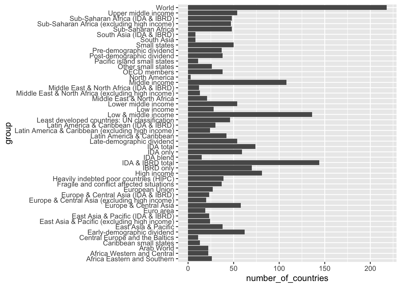

Let us find out how many groups each country belongs to.

wb_groups %>% group_by(country) %>% summarize(number_of_groups = n_distinct(group)) %>% arrange(desc(number_of_groups)) %>% DT::datatable()

From this we find that each country is classified into several groups.

5.4.1.2 Just for Fun

We use an intermediate level skill of defining a function in this subsection.

Let us make a list of iso3c codes each country belongs to. As we have seen above, Comoros belongs to 17 groups.

wb_groups %>% filter(country == "Comoros") %>% select(gcode, group) %>% DT::datatable()

wb_groups %>% filter(country == "Comoros") %>% pull(gcode) %>% paste(collapse = ", ")

## [1] "ARB, HPC, IBT, IDA, IDX, LDC, OSS, PRE, SSF, SST, TSS, WLD, AFE, FCS, LMC, LMY, MIC, SSA"

cd <- function(x){wb_groups %>% filter(country == x) %>%  pull(gcode) %>% paste(collapse = ", ")}
cd("Japan")

## [1] "EAS, OED, PST, WLD, OED, HIC"

cd("Comoros")

## [1] "ARB, HPC, IBT, IDA, IDX, LDC, OSS, PRE, SSF, SST, TSS, WLD, AFE, FCS, LMC, LMY, MIC, SSA"

cd("Zimbabwe")

## [1] "EAR, IBT, IDA, IDB, SSF, TSS, WLD, AFE, FCS, LMC, LMY, MIC, SSA"

cd("Pakistan")

## [1] "EAR, IBT, IDA, IDB, SAS, TSA, WLD, LMC, LMY, MIC"

wb_groups %>% group_by(country) %>% summarize(group_codes = cd(country)) %>% DT::datatable()

On the right of the table, you can find a list of group codes of each country.

5.5 Examples and Comments

In the following I include my feedback keeping anonymity.

5.5.1 Information Obtained by extra = TRUE

The first way is to use the option extra = TRUE when you import the data using WDI.

5.5.1.1 Population of Zimbabwe and Similar Countries

df_population <- as_tibble(WDI(
  country = "all",
  indicator = c(population = "SP.POP.TOTL"),
  start = 1960,
  end = 2020,
  extra = TRUE
))
DT::datatable(df_population)

## Warning in instance$preRenderHook(instance): It seems your data is too big
## for client-side DataTables. You may consider server-side processing: https://
## rstudio.github.io/DT/server.html

Find out extra information on Zimbabwe, i.e., which group Zimbabwe is in for region, income and lending.

df_population %>%
  filter(country == "Zimbabwe") %>% select(region, income, lending) %>% distinct()

## # A tibble: 1 × 3
##   region             income              lending
##   <chr>              <chr>               <chr>  
## 1 Sub-Saharan Africa Lower middle income Blend

Find out all countries in the same groups as Zimbabwe.

df_population %>% 
  filter(region == "Sub-Saharan Africa", income == "Lower middle income", lending == "Blend") %>% distinct(country)

## # A tibble: 6 × 1
##   country    
##   <chr>      
## 1 Cabo Verde 
## 2 Cameroon   
## 3 Congo, Rep.
## 4 Kenya      
## 5 Nigeria    
## 6 Zimbabwe

Since there are only 6 countries belonging to the same group as Zimbabwe, let us widen our search.

df_population %>% 
  filter(region == "Sub-Saharan Africa", income == "Lower middle income") %>% distinct(country)

## # A tibble: 17 × 1
##    country              
##    <chr>                
##  1 Angola               
##  2 Benin                
##  3 Cabo Verde           
##  4 Cameroon             
##  5 Comoros              
##  6 Congo, Rep.          
##  7 Cote d'Ivoire        
##  8 Eswatini             
##  9 Ghana                
## 10 Kenya                
## 11 Lesotho              
## 12 Mauritania           
## 13 Nigeria              
## 14 Sao Tome and Principe
## 15 Senegal              
## 16 Tanzania             
## 17 Zimbabwe

The following is the first chart.

df_population %>% 
  filter(region == "Sub-Saharan Africa", income == "Lower middle income", lending == "Blend") %>%
  ggplot() +
  geom_line(aes(x = year, y = population, color = country)) +
  scale_y_log10()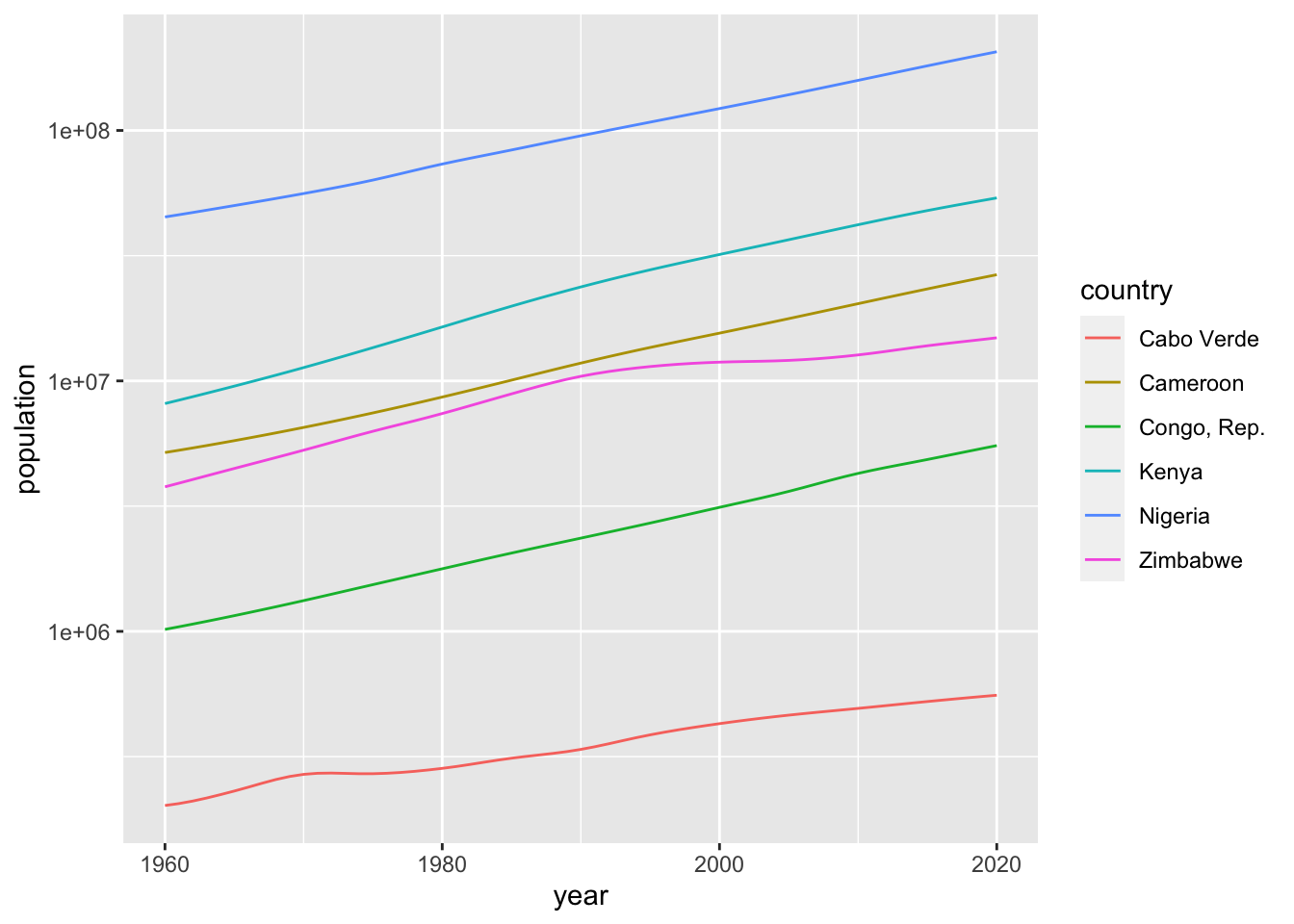

The second chart.

df_population %>% 
  filter(region == "Sub-Saharan Africa", income == "Lower middle income") %>%
  ggplot() +
  geom_line(aes(x = year, y = population, color = country)) +
  scale_y_log10()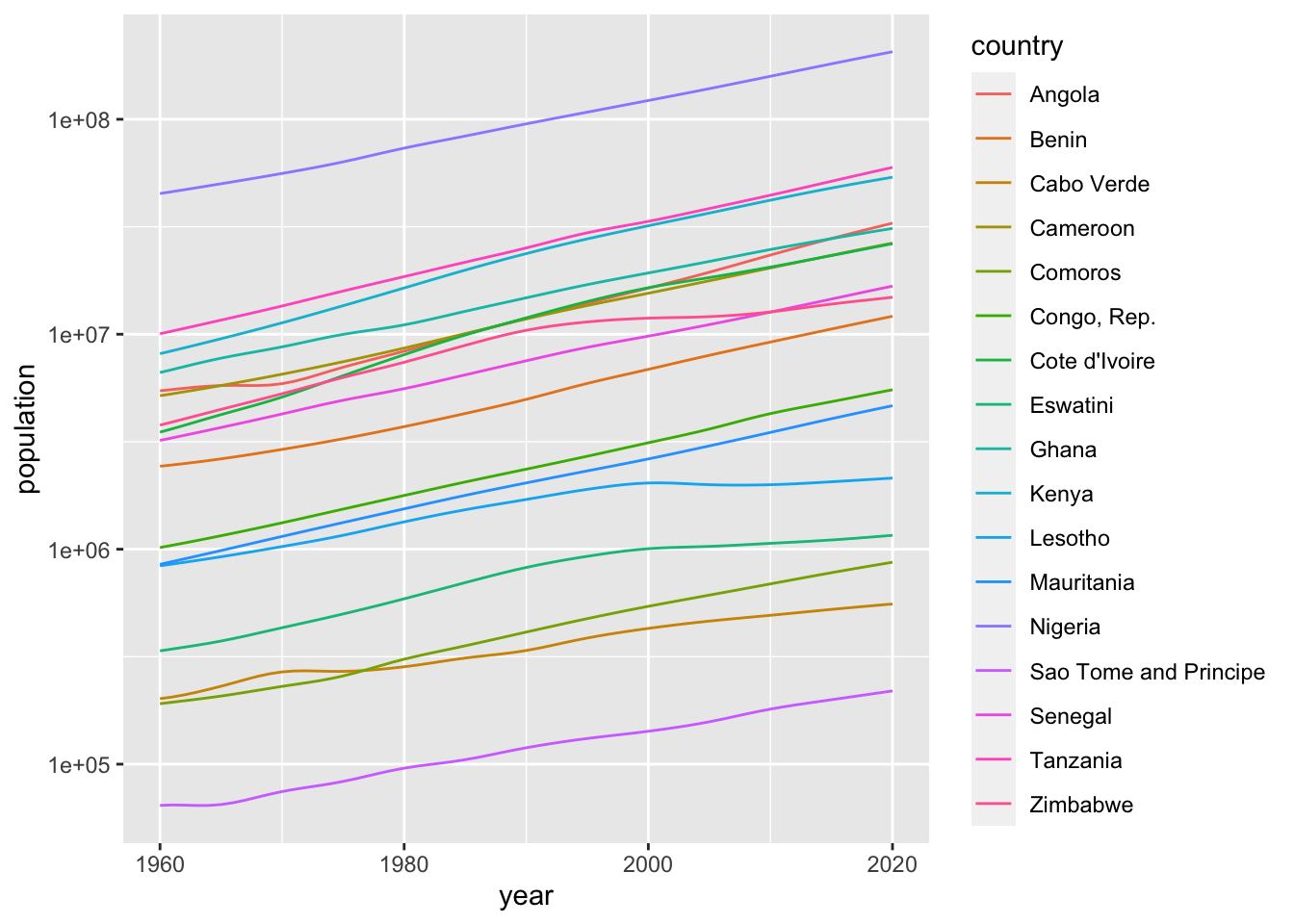

Fixing the income level and compare the regions.

df_population %>% filter(income == "Lower middle income")  %>%
  group_by(region, year) %>% 
  summarize(average_in_region = mean(population, na.rm = TRUE)) %>%
  ggplot() +
  geom_line(aes(x = year, y = average_in_region, color = region))

## `summarise()` has grouped output by 'region'. You can override using the
## `.groups` argument.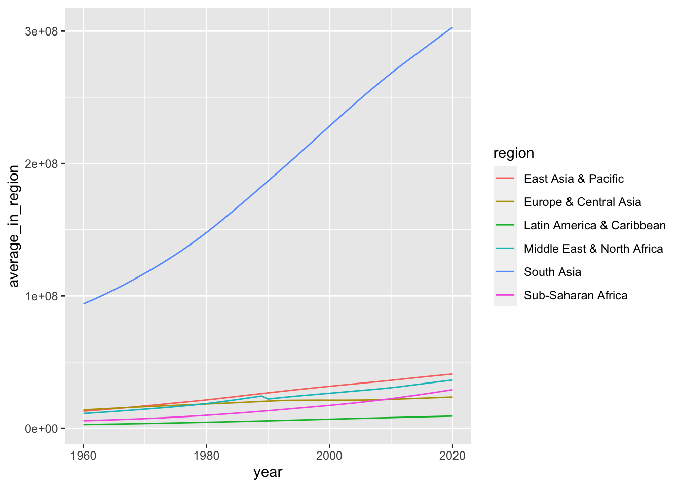

A chart in log 10 scale.

df_population %>% filter(income == "Lower middle income")  %>%
  group_by(region, year) %>% 
  summarize(average_in_region = mean(population, na.rm = TRUE)) %>%
  ggplot() +
  geom_line(aes(x = year, y = average_in_region, color = region)) +
  scale_y_log10()

## `summarise()` has grouped output by 'region'. You can override using the
## `.groups` argument.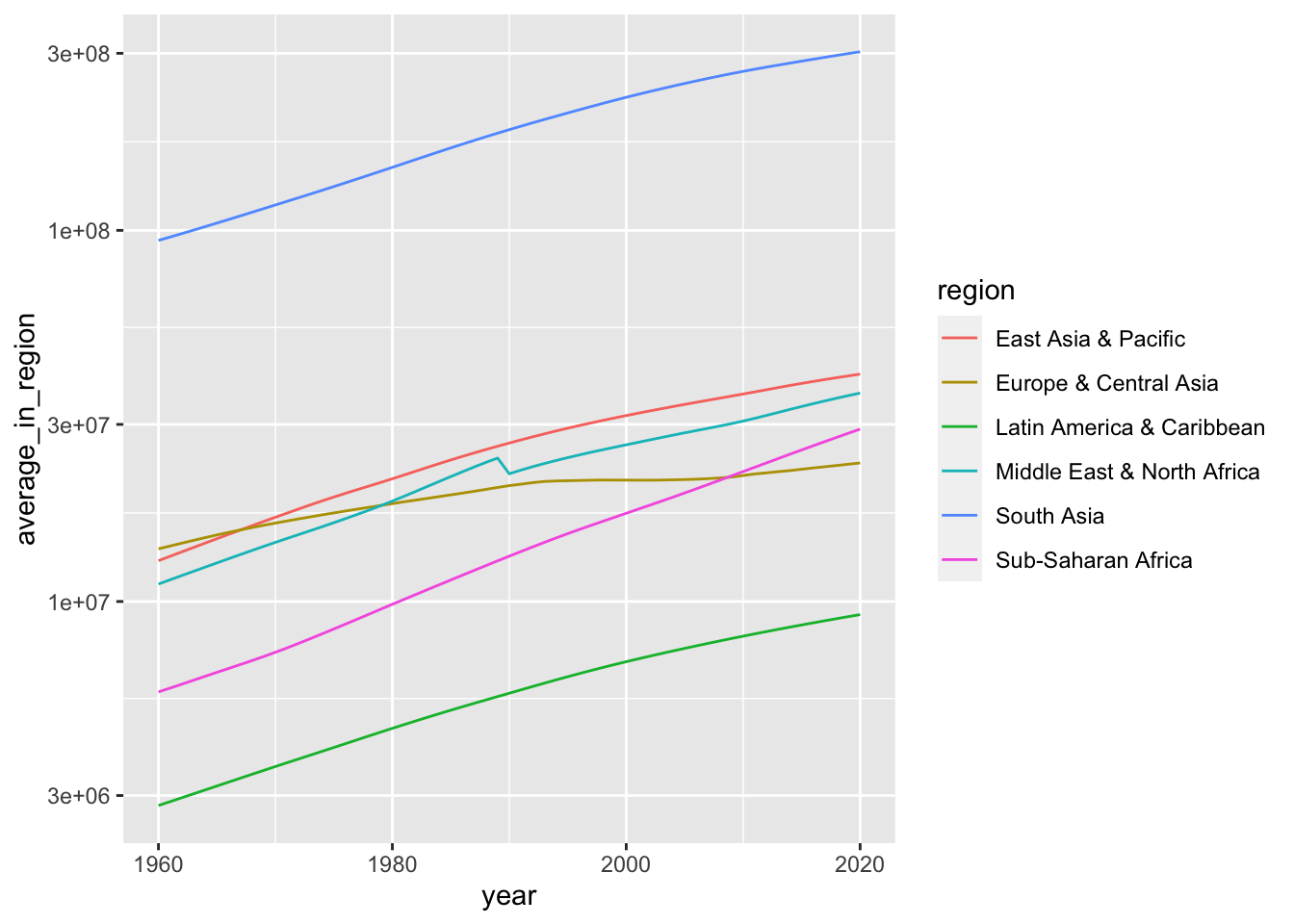

5.5.1.2 Fertility Rate of Japan and Similar Countries

df_fertility <- as_tibble(WDI(
  country = "all",
  indicator = c(fertility = "SP.DYN.TFRT.IN"), 
  start = 1960,
  end = 2020,
  extra = TRUE))
DT::datatable(df_fertility)

## Warning in instance$preRenderHook(instance): It seems your data is too big
## for client-side DataTables. You may consider server-side processing: https://
## rstudio.github.io/DT/server.html

df_fertility %>% filter(country == "Japan") %>%
  select(region, income, lending) %>% distinct()

## # A tibble: 1 × 3
##   region              income      lending       
##   <chr>               <chr>       <chr>         
## 1 East Asia & Pacific High income Not classified

Let us compare Japan’s fertility rate with similar countries, i.e., high income countries in East Asia & Pacific

df_fertility %>% filter(region == "East Asia & Pacific", income == "High income") %>% distinct(country)

## # A tibble: 13 × 1
##    country                 
##    <chr>                   
##  1 Australia               
##  2 Brunei Darussalam       
##  3 French Polynesia        
##  4 Guam                    
##  5 Hong Kong SAR, China    
##  6 Japan                   
##  7 Korea, Rep.             
##  8 Macao SAR, China        
##  9 Nauru                   
## 10 New Caledonia           
## 11 New Zealand             
## 12 Northern Mariana Islands
## 13 Singapore

df_fertility %>% filter(region == "East Asia & Pacific", income == "High income")  %>%
  ggplot() + 
  geom_line(aes(x = year, y = fertility, color = country)) +
  labs(title = "Fertility Rate of High Income Countries in East Asia & Pacific")

## Warning: Removed 122 rows containing missing values (`geom_line()`).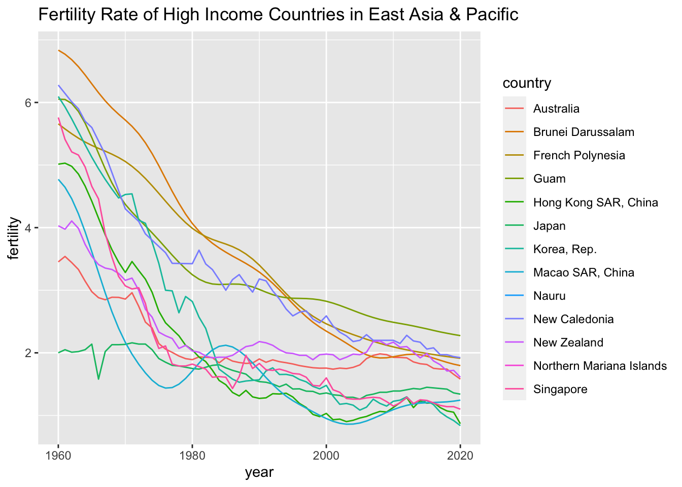

Let us check the number of countries in each region.

df_fertility %>% filter(income == "High income")  %>%
  select(country, region) %>% distinct() %>%
  group_by(region) %>% summarize(number_of_countries = n_distinct(country))

## # A tibble: 6 × 2
##   region                     number_of_countries
##   <chr>                                    <int>
## 1 East Asia & Pacific                         13
## 2 Europe & Central Asia                       37
## 3 Latin America & Caribbean                   17
## 4 Middle East & North Africa                   8
## 5 North America                                3
## 6 Sub-Saharan Africa                           1

df_fertility %>% filter(income == "High income")  %>%
  group_by(region, year) %>% 
  summarize(average_in_region = mean(fertility, na.rm = TRUE)) %>%
  ggplot() +
  geom_line(aes(x = year, y = average_in_region, color = region))

## `summarise()` has grouped output by 'region'. You can override using the
## `.groups` argument.

## Warning: Removed 16 rows containing missing values (`geom_line()`).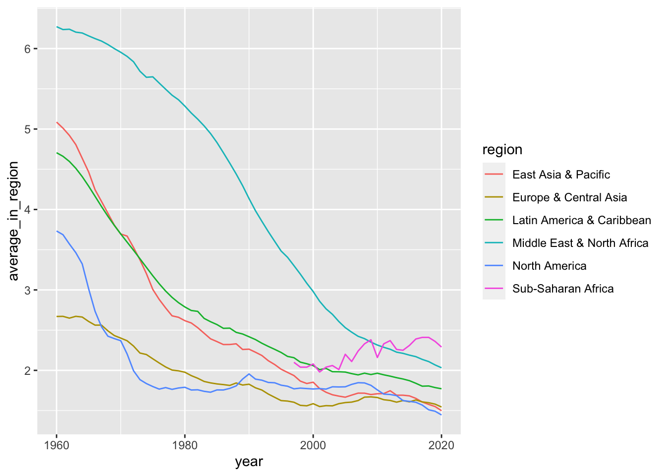

5.5.2 Other Groups

So far we used only three classifications of groups, region, income and lending. However, CLASS.xls contains more information.

For example if we compare data within a group, say Arab World (ARB), we need the information taken from CLASS.xlsx. If you need the information of the aggregated data of the group, it is included. We know that there are 22 countries.

wb_arb <- wb_groups %>% filter(gcode == "ARB") %>% select(iso3c, country)
wb_arb_vec <- wb_arb %>% pull(iso3c)
wb_arb

## # A tibble: 22 × 2
##    iso3c country             
##    <chr> <chr>               
##  1 ARE   United Arab Emirates
##  2 BHR   Bahrain             
##  3 COM   Comoros             
##  4 DJI   Djibouti            
##  5 DZA   Algeria             
##  6 EGY   Egypt, Arab Rep.    
##  7 IRQ   Iraq                
##  8 JOR   Jordan              
##  9 KWT   Kuwait              
## 10 LBN   Lebanon             
## # … with 12 more rows

wb_arb_vec

##  [1] "ARE" "BHR" "COM" "DJI" "DZA" "EGY" "IRQ" "JOR" "KWT" "LBN" "LBY" "MAR"
## [13] "MRT" "OMN" "PSE" "QAT" "SAU" "SDN" "SOM" "SYR" "TUN" "YEM"

I created the data frame containing Arab World countries and their iso3c codes together with a vector containing iso3c only.

5.5.2.1 iso3c vector: wb_arb_vec

df_fertility %>% filter(iso3c %in% wb_arb_vec) %>%
  ggplot(aes(x = year, y = fertility, color = country)) +
  geom_line()

## Warning: Removed 30 rows containing missing values (`geom_line()`).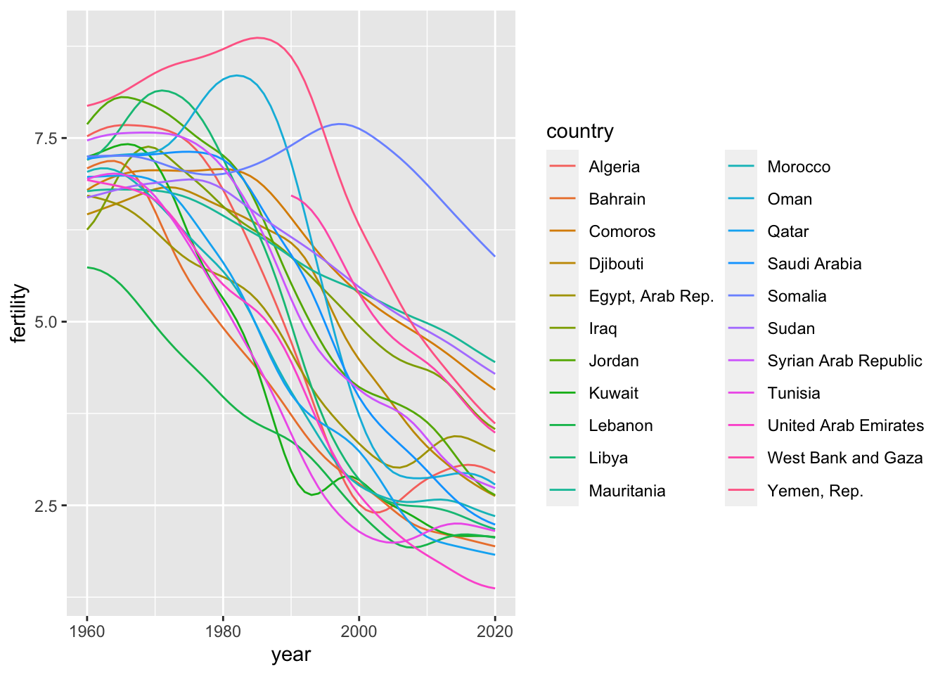

#### Data Frame: wb_arb

For example, if the original data does not have an iso3c code, you can obtain a part of data refering to the column they share in common. In the following I used by = "country" in the second code chunk.

df_fertility %>% right_join(wb_arb) %>%
  ggplot(aes(x = year, y = fertility, color = country)) +
  geom_line() + 
  labs(title = "right_join without using by")

## Joining, by = c("country", "iso3c")

## Warning: Removed 30 rows containing missing values (`geom_line()`).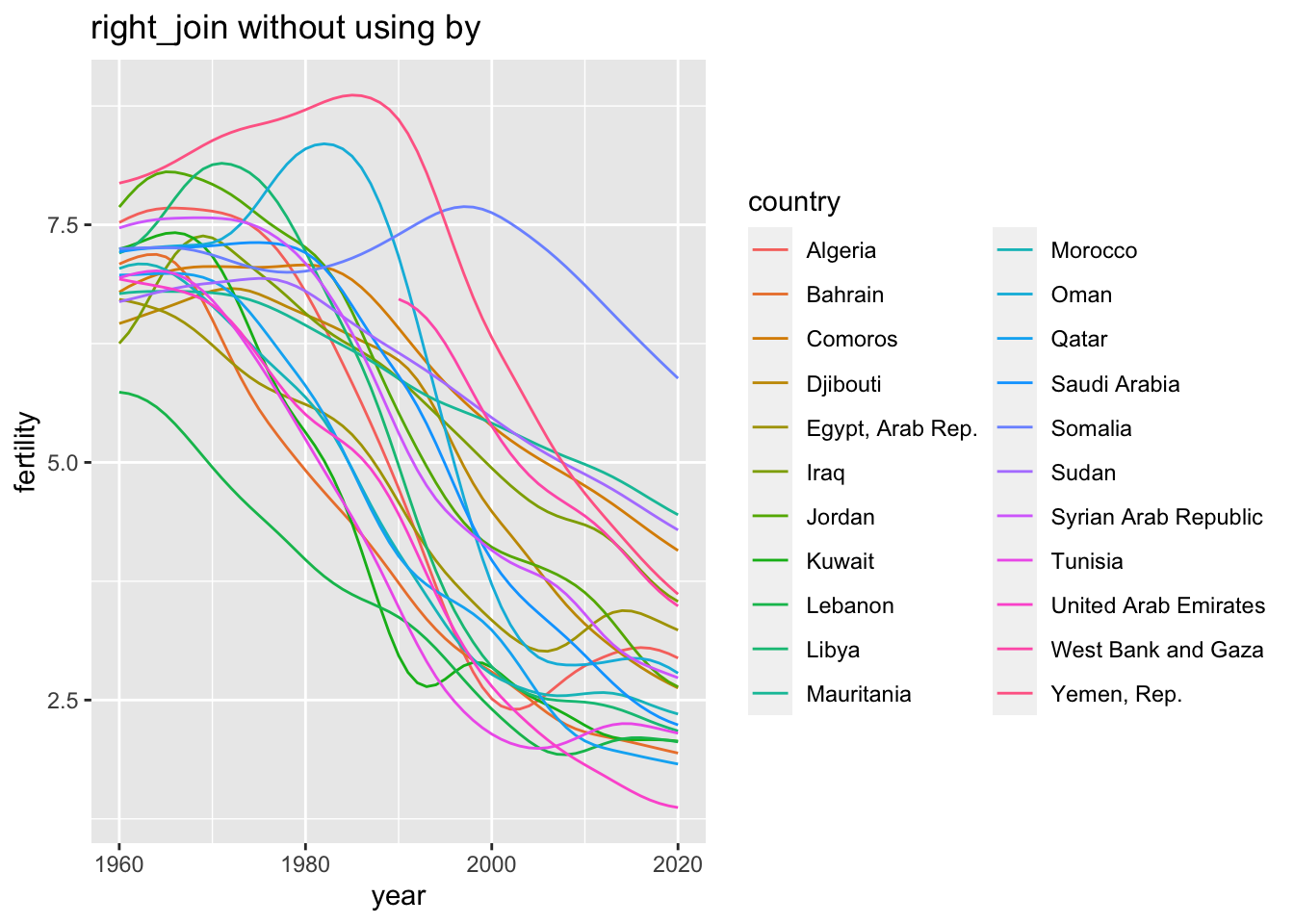

df_fertility %>% right_join(wb_arb, by = "country") %>%
  ggplot(aes(x = year, y = fertility, color = country)) +
  geom_line()  + 
  labs(title = "`right_join` with `by`")

## Warning: Removed 30 rows containing missing values (`geom_line()`).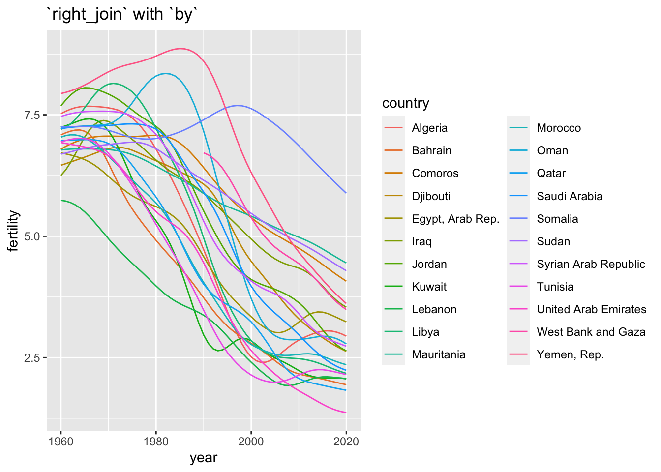

5.5.3 Wangling: Transform and Tidy Data

url_class <- "https://api.worldbank.org/v2/en/indicator/EN.ATM.CO2E.PC?downloadformat=excel"
download.file(url = url_class, mode = "wb", destfile = "data/API_EN.ATM.CO2E.PC_DS2_en_excel_v2_3469464.xls")

5.5.3.1 Tidying data

country_tmp <- read_excel("data/API_EN.ATM.CO2E.PC_DS2_en_excel_v2_3469464.xls", sheet = 1, skip = 3, n_max =271) %>% slice(-1)

DT::datatable(country_tmp)

The following is an original code chunk.

Co2_country <- country_tmp %>%
  select(`Country Name`, `Country Code`, `Indicator Name`, `Indicator Code`,`1960`:`2018`)
Co2_country <- pivot_longer(Co2_country,cols = 5:63, names_to = "year", values_to = "Co2", values_drop_na = TRUE) %>%
  select(ID = `Country Code`, Country = `Country Name`, year, Co2)
DT::datatable(Co2_country)

Co2_country %>% filter(ID == "WLD") %>% 
  ggplot(aes(x = year, y = Co2)) +
  geom_line()

## `geom_line()`: Each group consists of only one observation.
## ℹ Do you need to adjust the group aesthetic?

Empty chart. The following is much better but we cannot see year and a line graph may be preferable to see changes. Please notice that year is in character not in integer.

Co2_country %>% filter(ID == "WLD") %>% 
  ggplot(aes(x = year, y = Co2)) +
  geom_point()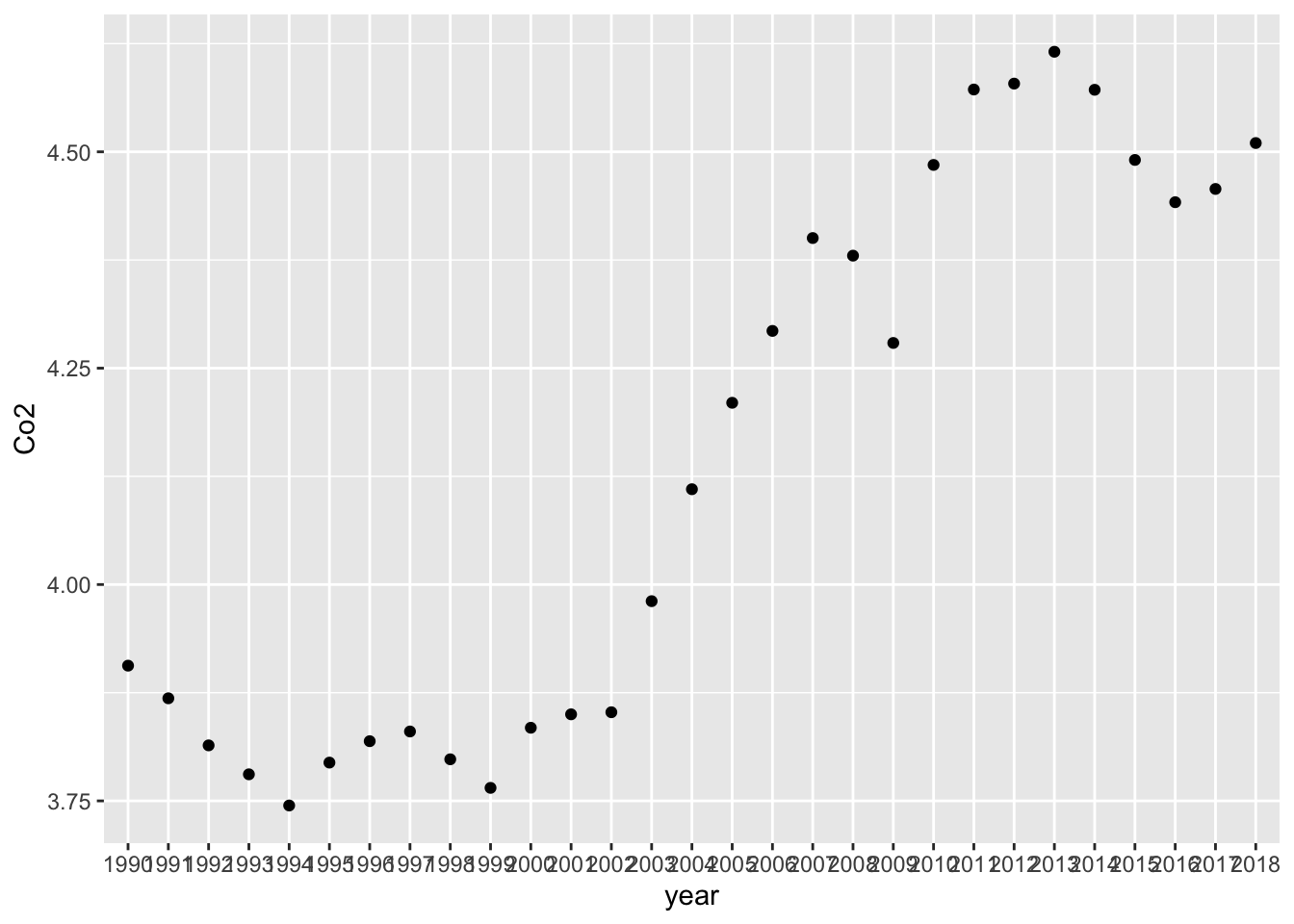

In the following I used Base R command. Co2_country_rev$year denotes the column year of the data frame Co2_country_rev.

Co2_country_rev <- Co2_country
Co2_country_rev$year <- as.integer(Co2_country_rev$year) 
Co2_country_rev %>% filter(ID == "WLD") %>% 
  ggplot(aes(x = year, y = Co2)) +
  geom_line()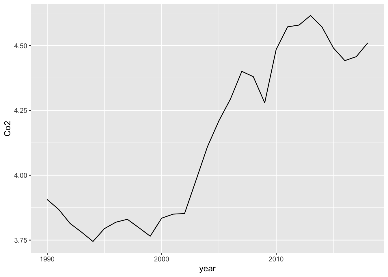

Using dplyr, the following is an alternative.

Co2_country_rev2 <- Co2_country %>% mutate(year = as.integer(year))
Co2_country_rev2 %>% filter(ID == "WLD") %>% 
  ggplot(aes(x = year, y= Co2)) +
  geom_line()

It is possible to set year to be an integer variable when pivot_longer is applied by adding names_transform = list(year = as.integer).

co2_country <- country_tmp %>%
  select('Country Name', 'Country Code', 'Indicator Name', 'Indicator Code','1960':'2018')
co2_country <- pivot_longer(co2_country,cols = 5:63, names_to = "year", names_transform = list(year = as.integer), values_to = "Co2", values_drop_na = TRUE) %>%
  select(ID = 'Country Code', Country = 'Country Name', year, Co2)
DT::datatable(co2_country)

co2_country <- country_tmp %>% 
  pivot_longer(cols = 5:63, names_to = "year", names_transform = list(year = as.integer), 
               values_to = "co2", values_drop_na = TRUE) %>%
  select(id = 'Country Code', country = 'Country Name', year, co2)
DT::datatable(co2_country)

co2_country %>% filter(id %in% c("WLD", "USA", "CHN", "JPN")) %>% 
  ggplot(aes(x = year, y= co2, color = id)) +
  geom_line()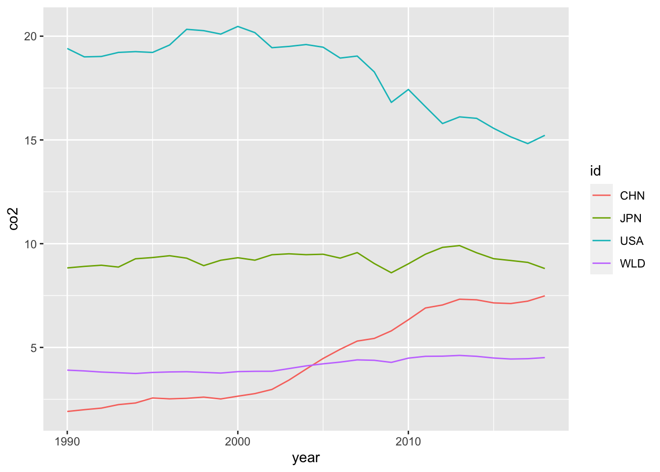

COUNTRIES <- c("China","Japan","United States","Great Britain","India","South Africa","Malaysia","Russia","Australia", "Canada", "Vietnam")
co2_country %>% filter(country %in% COUNTRIES) %>% 
  ggplot(aes(x = year, y= co2, color = country)) +
  geom_line() +
  geom_point()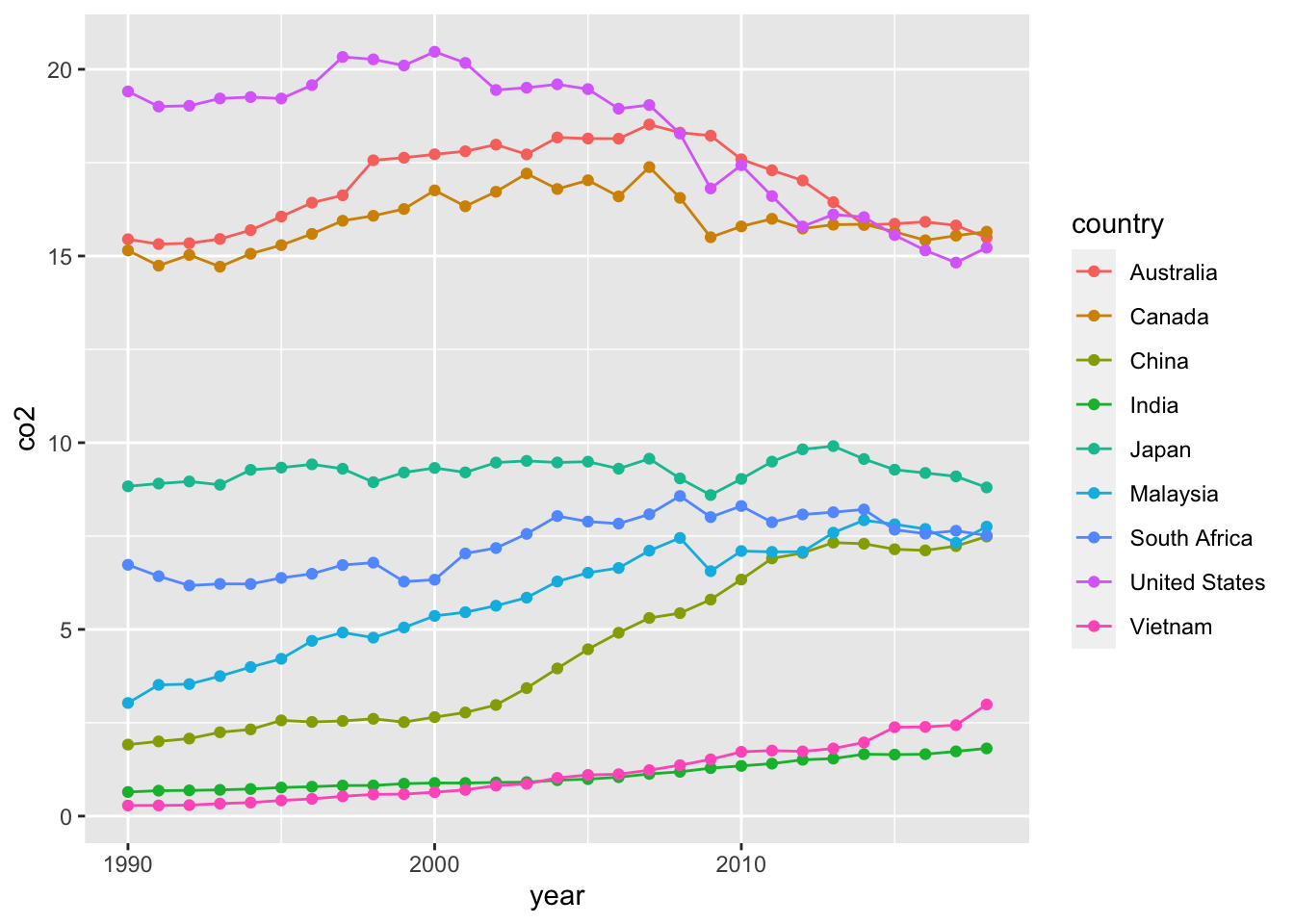

Compare the data above and the those in WDI.

• WID Data
• URL: https://data.worldbank.org/indicator/EN.ATM.CO2E.KT
• Description:

WDIsearch(string = "co2", field = "name") %>% DT::datatable()

5.5.4 Population Analysis

The original analysis uses Base R commands a lot, I do a similar analysis using tidyverse as an example.

The following population data has seven variables.

url <- "https://data.un.org/_Docs/SYB/CSV/SYB64_246_202110_Population%20Growth,%20Fertility%20and%20Mortality%20Indicators.csv"
df_un_pop <- read_csv(url, skip = 1)

## New names:
## • `` -> `...2`

## Warning: One or more parsing issues, call `problems()` on your data frame for details, e.g.:
##   dat <- vroom(...)
##   problems(dat)

## Rows: 4899 Columns: 7
## ── Column specification ──────────────────────────────────────────────────────────────────────────────────────────────────────
## Delimiter: ","
## chr (4): ...2, Series, Footnotes, Source
## dbl (3): Region/Country/Area, Year, Value
## 
## ℹ Use `spec()` to retrieve the full column specification for this data.
## ℹ Specify the column types or set `show_col_types = FALSE` to quiet this message.

df_un_pop

## # A tibble: 4,899 × 7
##    `Region/Country/Area` ...2                   Year Series Value Footn…¹ Source
##                    <dbl> <chr>                 <dbl> <chr>  <dbl> <chr>   <chr> 
##  1                     1 Total, all countries…  2010 Popul…   1.2 Data r… "Unit…
##  2                     1 Total, all countries…  2010 Total…   2.6 Data r… "Unit…
##  3                     1 Total, all countries…  2010 Infan…  41   Data r… "Unit…
##  4                     1 Total, all countries…  2010 Mater… 248   <NA>    "Worl…
##  5                     1 Total, all countries…  2010 Life …  68.9 Data r… "Unit…
##  6                     1 Total, all countries…  2010 Life …  66.7 Data r… "Unit…
##  7                     1 Total, all countries…  2010 Life …  71.3 Data r… "Unit…
##  8                     1 Total, all countries…  2015 Popul…   1.2 Data r… "Unit…
##  9                     1 Total, all countries…  2015 Total…   2.5 Data r… "Unit…
## 10                     1 Total, all countries…  2015 Infan…  33.9 Data r… "Unit…
## # … with 4,889 more rows, and abbreviated variable name ¹​Footnotes

Check the regions of interst.

df_un_pop %>% filter(`Region/Country/Area` %in% c(2,9,21,419,142,150)) %>% distinct(`...2`)

## # A tibble: 6 × 1
##   ...2                         
##   <chr>                        
## 1 Africa                       
## 2 Northern America             
## 3 Latin America & the Caribbean
## 4 Asia                         
## 5 Europe                       
## 6 Oceania

df_un_pop_rev <- df_un_pop %>% 
  select(rn = `Region/Country/Area`, region = `...2`, year = Year, series = Series, value = Value) %>%
  filter(rn %in% c(2,9,21,419,142,150))
DT::datatable(df_un_pop_rev)

df_un_pop_rev %>% distinct(series)

## # A tibble: 7 × 1
##   series                                                  
##   <chr>                                                   
## 1 Population annual rate of increase (percent)            
## 2 Total fertility rate (children per women)               
## 3 Infant mortality for both sexes (per 1,000 live births) 
## 4 Life expectancy at birth for both sexes (years)         
## 5 Life expectancy at birth for males (years)              
## 6 Life expectancy at birth for females (years)            
## 7 Maternal mortality ratio (deaths per 100,000 population)

df_un_pop_rev %>% filter(series == "Population annual rate of increase (percent)") %>%
  ggplot(aes(x = year, y = value, color = region)) + 
  geom_line() +
  labs(title = "Population annual rate of increase (percent)")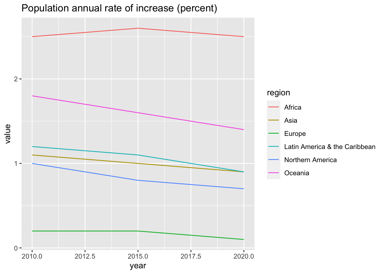

df_un_pop_rev %>% filter(series == "Total fertility rate (children per women)") %>%
  ggplot(aes(x = year, y = value, color = region)) + 
  geom_line() +
  labs(title = "Total fertility rate (children per women)")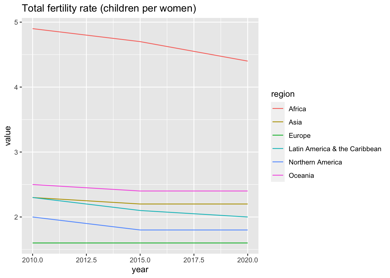

df_un_pop_rev %>% filter(series == "Infant mortality for both sexes (per 1,000 live births)") %>%
  ggplot(aes(x = year, y = value, color = region)) + 
  geom_line() +
  labs(title = "Infant mortality for both sexes (per 1,000 live births)")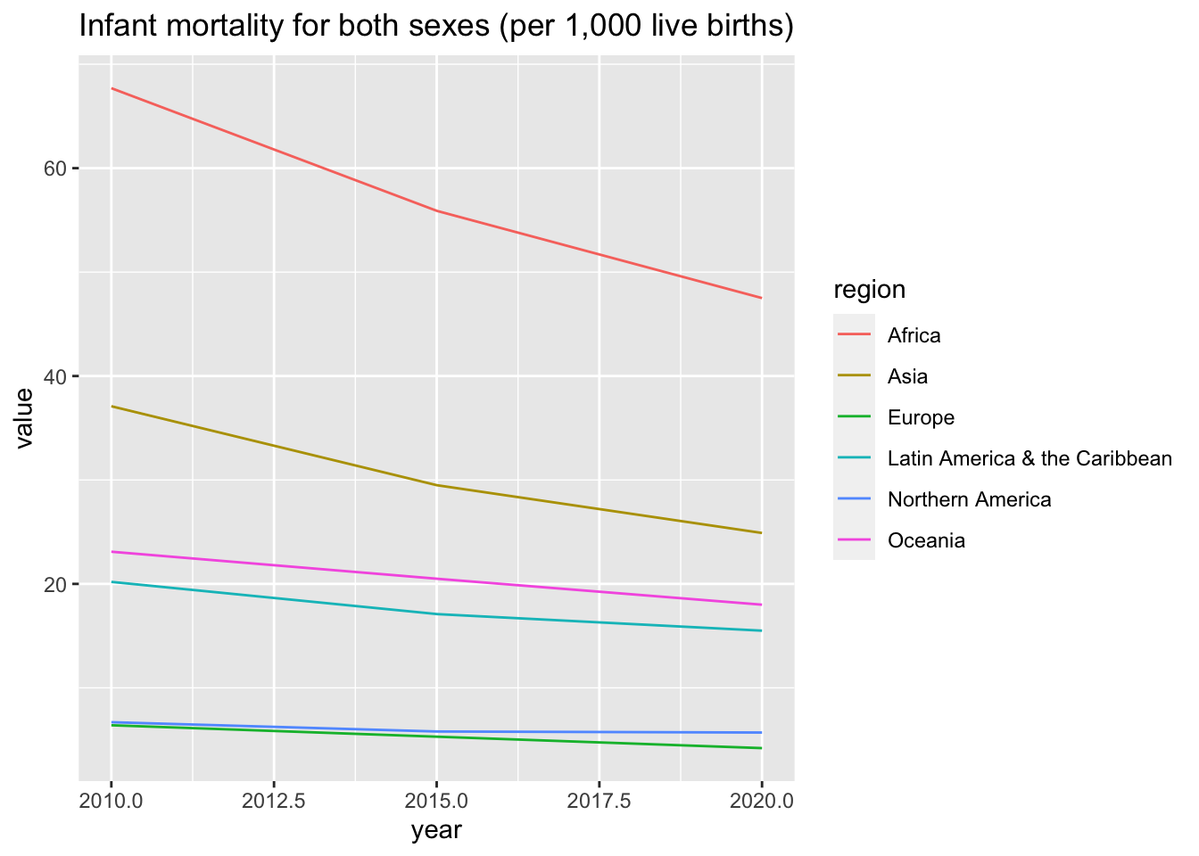

5.5.5 Literacy rate, youth total (% of people ages 15-24)

I will introduce this because it uses semi_join to choose countries’ data deleting aggrigated data.

WDIsearch(string = "SE.ADT.1524.LT.ZS", field = "indicator", cache = NULL)

##               indicator                                                name
## 15166 SE.ADT.1524.LT.ZS Literacy rate, youth total (% of people ages 15-24)

literacy_rate_youth <- WDI(country = "all", indicator = "SE.ADT.1524.LT.ZS")
DT::datatable(literacy_rate_youth)

## Warning in instance$preRenderHook(instance): It seems your data is too big
## for client-side DataTables. You may consider server-side processing: https://
## rstudio.github.io/DT/server.html

5.5.5.1 Filtering joins

Description

Filtering joins filter rows from x based on the presence or absence of matches in y:

• semi_join() return all rows from x with a match in y.

• anti_join() return all rows from x without a match in y.

• Combine the literacy rate data with the country data

  • semi_joint: list contains countries only listed in wb_countries
  • deleted some of the aggregated data

literacy_rate_youth_country <- literacy_rate_youth %>% semi_join(wb_countries, by = "country")
DT::datatable(literacy_rate_youth_country)

Compare with the following.

literacy_rate_youth_aggregated <- literacy_rate_youth %>% anti_join(wb_countries, by = "country")
DT::datatable(literacy_rate_youth_aggregated)

5.5.6 Visualization of the data

5.5.6.1 Gender: Ratio of girls to boys in primary, secondary and tertiary levels

• Went to http://data.un.org/ (UNdata website)
• Scrolled down to “Gender” within “Popular statistical tables, country (area) and regional profiles”
• Copied CSV download link for “Ratio of girls to boys in primary, secondary and tertiary levels”
• Pasted the link below⇩

url_of_data <- "http://data.un.org/_Docs/SYB/CSV/SYB64_319_202110_Ratio%20of%20girls%20to%20boys%20in%20education.csv"

gender_education <- read_csv("http://data.un.org/_Docs/SYB/CSV/SYB64_319_202110_Ratio%20of%20girls%20to%20boys%20in%20education.csv", skip = 1)

## New names:
## Rows: 2881 Columns: 7
## ── Column specification
## ──────────────────────────────────────────────────────────────────────────────────────────────────────
## Delimiter: "," chr (4): ...2, Series, Footnotes, Source dbl (3): Region/Country/Area, Year, Value
## ℹ Use `spec()` to retrieve the full column specification for this data. ℹ Specify the column types or set `show_col_types =
## FALSE` to quiet this message.
## • `` -> `...2`

gender_education

## # A tibble: 2,881 × 7
##    `Region/Country/Area` ...2                   Year Series Value Footn…¹ Source
##                    <dbl> <chr>                 <dbl> <chr>  <dbl> <chr>   <chr> 
##  1                     1 Total, all countries…  1995 Ratio…  0.91 <NA>    Unite…
##  2                     1 Total, all countries…  2005 Ratio…  0.95 <NA>    Unite…
##  3                     1 Total, all countries…  2010 Ratio…  0.97 <NA>    Unite…
##  4                     1 Total, all countries…  2015 Ratio…  1    <NA>    Unite…
##  5                     1 Total, all countries…  2017 Ratio…  1    <NA>    Unite…
##  6                     1 Total, all countries…  2018 Ratio…  0.98 <NA>    Unite…
##  7                     1 Total, all countries…  2019 Ratio…  0.98 Estima… Unite…
##  8                     1 Total, all countries…  1995 Ratio…  0.88 <NA>    Unite…
##  9                     1 Total, all countries…  2005 Ratio…  0.95 <NA>    Unite…
## 10                     1 Total, all countries…  2010 Ratio…  0.97 <NA>    Unite…
## # … with 2,871 more rows, and abbreviated variable name ¹​Footnotes

colnames(gender_education)

## [1] "Region/Country/Area" "...2"                "Year"               
## [4] "Series"              "Value"               "Footnotes"          
## [7] "Source"

It is a good try to use pivot_wider, and it is easy to see the data. However for visualization using tidyverse it is not necessary if you use filter and/or grouping.

gender_education_tbl <- gender_education %>% select(num = "Region/Country/Area", region = "...2", year = "Year", series = "Series", value = "Value") %>% 
  pivot_wider(names_from = series, values_from = value) 
gender_education_tbl

## # A tibble: 1,173 × 6
##      num region                         year Ratio of girls to…¹ Ratio…² Ratio…³
##    <dbl> <chr>                         <dbl>               <dbl>   <dbl>   <dbl>
##  1     1 Total, all countries or areas  1995                0.91    0.88    0.95
##  2     1 Total, all countries or areas  2005                0.95    0.95    1.05
##  3     1 Total, all countries or areas  2010                0.97    0.97    1.07
##  4     1 Total, all countries or areas  2015                1       0.99    1.1 
##  5     1 Total, all countries or areas  2017                1       0.99    1.12
##  6     1 Total, all countries or areas  2018                0.98    0.99    1.12
##  7     1 Total, all countries or areas  2019                0.98    0.99    1.13
##  8    15 Northern Africa                1995                0.86    0.86    0.76
##  9    15 Northern Africa                2005                0.93    0.99    0.96
## 10    15 Northern Africa                2010                0.95    0.98    1.07
## # … with 1,163 more rows, and abbreviated variable names
## #   ¹​`Ratio of girls to boys in primary education`,
## #   ²​`Ratio of girls to boys in secondary education`,
## #   ³​`Ratio of girls to boys in tertiary education`

5.5.6.1.1 Visualization

The student asks: I do not know how to visualize this data using ggplot…

1. First select one region and make a scatter plot and see the data.

gender_education %>% filter(`Region/Country/Area` == 1) %>%  
  ggplot() +
  geom_point(aes(x = Year, y = Value))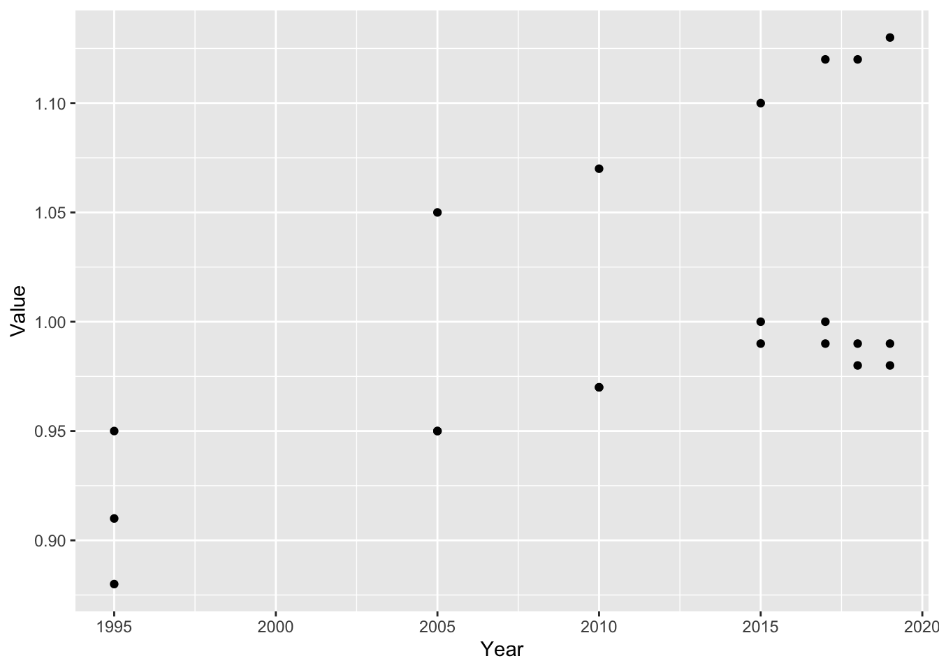

2. Since there are a few data in each year, use color and geom_line as well.

gender_education %>% filter(`Region/Country/Area` == 1) %>%  
  ggplot(aes(x = Year, y = Value, color = Series)) +
  geom_point() +
  geom_line()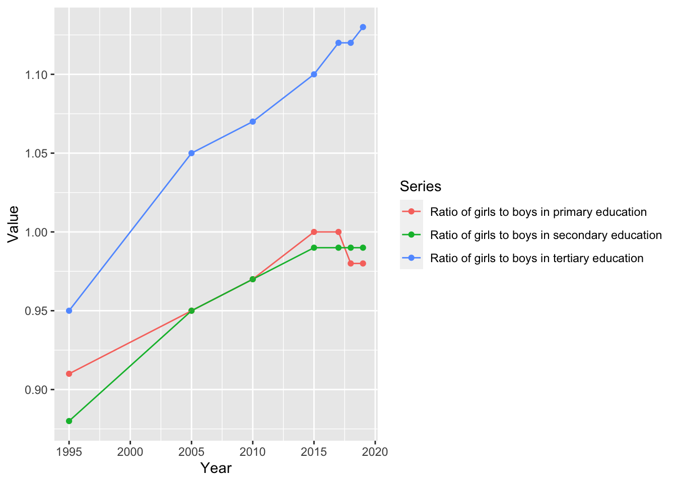

3. Now we choose several countries and start analyzing what you want. Probably it is easier to see in separate charts. I wanted to introduce facet-grid.

gender_education %>% 
  select(`Region/Country/Area`, region = `...2`, year = Year, value = Value, series = Series) %>%
  mutate(year = as.integer(year)) %>%
  filter(`Region/Country/Area` %in% c(1, 15, 202, 21, 419, 143, 30, 35, 34, 145, 150, 9)) %>%  
  ggplot(aes(x = year, y = value, color = region)) +
  geom_point() +
  geom_line() +
  facet_grid(cols = vars(series))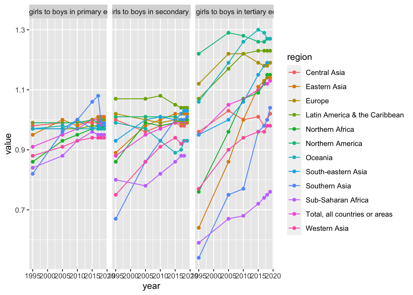

5.5.6.2 Proportion of seats held by women in national parliament.

url_of_df <- "http://data.un.org/_Docs/SYB/CSV/SYB64_317_202110_Seats%20held%20by%20women%20in%20Parliament.csv"
download.file(url = url_of_df, destfile = "data/UN_WO.csv")

df_UN_WO <- read_csv("data/UN_WO.csv", skip = 1)

## New names:
## Rows: 1958 Columns: 9
## ── Column specification
## ──────────────────────────────────────────────────────────────────────────────────────────────────────
## Delimiter: "," chr (5): ...2, Series, Last Election Date, Footnotes, Source dbl (3): Region/Country/Area, Year, Value lgl
## (1): Last Election Date footnote
## ℹ Use `spec()` to retrieve the full column specification for this data. ℹ Specify the column types or set `show_col_types =
## FALSE` to quiet this message.
## • `` -> `...2`

df_UN_WO

## # A tibble: 1,958 × 9
##    `Region/Country/Area` ...2   Year Series Last …¹ Last …² Value Footn…³ Source
##                    <dbl> <chr> <dbl> <chr>  <chr>   <lgl>   <dbl> <chr>   <chr> 
##  1                     1 Tota…  2000 Seats… <NA>    NA       13.3 <NA>    "Inte…
##  2                     1 Tota…  2005 Seats… <NA>    NA       15.9 <NA>    "Inte…
##  3                     1 Tota…  2010 Seats… <NA>    NA       19   <NA>    "Inte…
##  4                     1 Tota…  2015 Seats… <NA>    NA       22.3 <NA>    "Inte…
##  5                     1 Tota…  2017 Seats… <NA>    NA       23.4 <NA>    "Inte…
##  6                     1 Tota…  2018 Seats… <NA>    NA       23.4 <NA>    "Inte…
##  7                     1 Tota…  2019 Seats… <NA>    NA       24.3 <NA>    "Inte…
##  8                     1 Tota…  2020 Seats… <NA>    NA       24.9 Data a… "Inte…
##  9                     1 Tota…  2021 Seats… <NA>    NA       25.6 Data a… "Inte…
## 10                    15 Nort…  2000 Seats… <NA>    NA        5.4 <NA>    "Inte…
## # … with 1,948 more rows, and abbreviated variable names ¹​`Last Election Date`,
## #   ²​`Last Election Date footnote`, ³​Footnotes

colnames(df_UN_WO)

## [1] "Region/Country/Area"         "...2"                       
## [3] "Year"                        "Series"                     
## [5] "Last Election Date"          "Last Election Date footnote"
## [7] "Value"                       "Footnotes"                  
## [9] "Source"

UN_WO_tbl <- df_UN_WO %>% select(num = "Region/Country/Area", region = "...2", year = "Year", series = "Series", LED = "Last Election Date", value = "Value")%>%
pivot_wider (names_from = series, values_from = value) 
UN_WO_tbl

## # A tibble: 1,958 × 5
##      num region                         year LED   Seats held by women in nati…¹
##    <dbl> <chr>                         <dbl> <chr>                         <dbl>
##  1     1 Total, all countries or areas  2000 <NA>                           13.3
##  2     1 Total, all countries or areas  2005 <NA>                           15.9
##  3     1 Total, all countries or areas  2010 <NA>                           19  
##  4     1 Total, all countries or areas  2015 <NA>                           22.3
##  5     1 Total, all countries or areas  2017 <NA>                           23.4
##  6     1 Total, all countries or areas  2018 <NA>                           23.4
##  7     1 Total, all countries or areas  2019 <NA>                           24.3
##  8     1 Total, all countries or areas  2020 <NA>                           24.9
##  9     1 Total, all countries or areas  2021 <NA>                           25.6
## 10    15 Northern Africa                2000 <NA>                            5.4
## # … with 1,948 more rows, and abbreviated variable name
## #   ¹​`Seats held by women in national parliament, as of February (%)`

colnames(UN_WO_tbl) <- c("num", "region", "year", "LED", "seats")
UN_WO_tbl

## # A tibble: 1,958 × 5
##      num region                         year LED   seats
##    <dbl> <chr>                         <dbl> <chr> <dbl>
##  1     1 Total, all countries or areas  2000 <NA>   13.3
##  2     1 Total, all countries or areas  2005 <NA>   15.9
##  3     1 Total, all countries or areas  2010 <NA>   19  
##  4     1 Total, all countries or areas  2015 <NA>   22.3
##  5     1 Total, all countries or areas  2017 <NA>   23.4
##  6     1 Total, all countries or areas  2018 <NA>   23.4
##  7     1 Total, all countries or areas  2019 <NA>   24.3
##  8     1 Total, all countries or areas  2020 <NA>   24.9
##  9     1 Total, all countries or areas  2021 <NA>   25.6
## 10    15 Northern Africa                2000 <NA>    5.4
## # … with 1,948 more rows

UN_WO_tbl_short <- UN_WO_tbl %>% select(region, year, seats)
UN_WO_tbl_short

## # A tibble: 1,958 × 3
##    region                         year seats
##    <chr>                         <dbl> <dbl>
##  1 Total, all countries or areas  2000  13.3
##  2 Total, all countries or areas  2005  15.9
##  3 Total, all countries or areas  2010  19  
##  4 Total, all countries or areas  2015  22.3
##  5 Total, all countries or areas  2017  23.4
##  6 Total, all countries or areas  2018  23.4
##  7 Total, all countries or areas  2019  24.3
##  8 Total, all countries or areas  2020  24.9
##  9 Total, all countries or areas  2021  25.6
## 10 Northern Africa                2000   5.4
## # … with 1,948 more rows

UN_WO_tbl_short$year <- as.integer(UN_WO_tbl_short$year)
UN_WO_tbl_short

## # A tibble: 1,958 × 3
##    region                         year seats
##    <chr>                         <int> <dbl>
##  1 Total, all countries or areas  2000  13.3
##  2 Total, all countries or areas  2005  15.9
##  3 Total, all countries or areas  2010  19  
##  4 Total, all countries or areas  2015  22.3
##  5 Total, all countries or areas  2017  23.4
##  6 Total, all countries or areas  2018  23.4
##  7 Total, all countries or areas  2019  24.3
##  8 Total, all countries or areas  2020  24.9
##  9 Total, all countries or areas  2021  25.6
## 10 Northern Africa                2000   5.4
## # … with 1,948 more rows

5.5.6.2.1 Visualization

UN_WO_tbl_short %>% filter(year %in% c(2000, 2005, 2010, 2015, 2020)) %>% 
  mutate(year = as.factor(year)) %>%
  ggplot() +
  geom_freqpoly(aes(x = seats, color = year))

## `stat_bin()` using `bins = 30`. Pick better value with `binwidth`.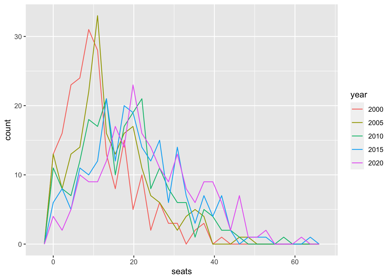

UN_WO_tbl_short %>% filter(year %in% c(2000, 2005, 2010, 2015, 2020)) %>% 
  mutate(year = as.factor(year)) %>%
  group_by(year) %>% count(cut_width(seats, 5))

## # A tibble: 57 × 3
## # Groups:   year [5]
##    year  `cut_width(seats, 5)`     n
##    <fct> <fct>                 <int>
##  1 2000  [-2.5,2.5]               24
##  2 2000  (2.5,7.5]                50
##  3 2000  (7.5,12.5]               65
##  4 2000  (12.5,17.5]              25
##  5 2000  (17.5,22.5]              21
##  6 2000  (22.5,27.5]               9
##  7 2000  (27.5,32.5]               6
##  8 2000  (32.5,37.5]               5
##  9 2000  (42.5,47.5]               1
## 10 2005  [-2.5,2.5]               17
## # … with 47 more rows

UN_WO_tbl_short

## # A tibble: 1,958 × 3
##    region                         year seats
##    <chr>                         <int> <dbl>
##  1 Total, all countries or areas  2000  13.3
##  2 Total, all countries or areas  2005  15.9
##  3 Total, all countries or areas  2010  19  
##  4 Total, all countries or areas  2015  22.3
##  5 Total, all countries or areas  2017  23.4
##  6 Total, all countries or areas  2018  23.4
##  7 Total, all countries or areas  2019  24.3
##  8 Total, all countries or areas  2020  24.9
##  9 Total, all countries or areas  2021  25.6
## 10 Northern Africa                2000   5.4
## # … with 1,948 more rows

wb_regions

## # A tibble: 45 × 2
##    region                                        iso3c
##    <chr>                                         <chr>
##  1 Caribbean small states                        CSS  
##  2 Central Europe and the Baltics                CEB  
##  3 Early-demographic dividend                    EAR  
##  4 East Asia & Pacific                           EAS  
##  5 East Asia & Pacific (excluding high income)   EAP  
##  6 East Asia & Pacific (IDA & IBRD)              TEA  
##  7 Euro area                                     EMU  
##  8 Europe & Central Asia                         ECS  
##  9 Europe & Central Asia (excluding high income) ECA  
## 10 Europe & Central Asia (IDA & IBRD)            TEC  
## # … with 35 more rows

UN_WO_tbl_short %>% filter(region %in% c("Total, all countries or areas", "Northern Africa", "Sub-Saharan Africa", "Eastern Africa", "Middle Africa", "Southern Africa", "Western Africa")) %>%
  ggplot() + geom_line(aes(x= year, y= seats, color= region)) + labs(title = "Seats of Women in Parliament")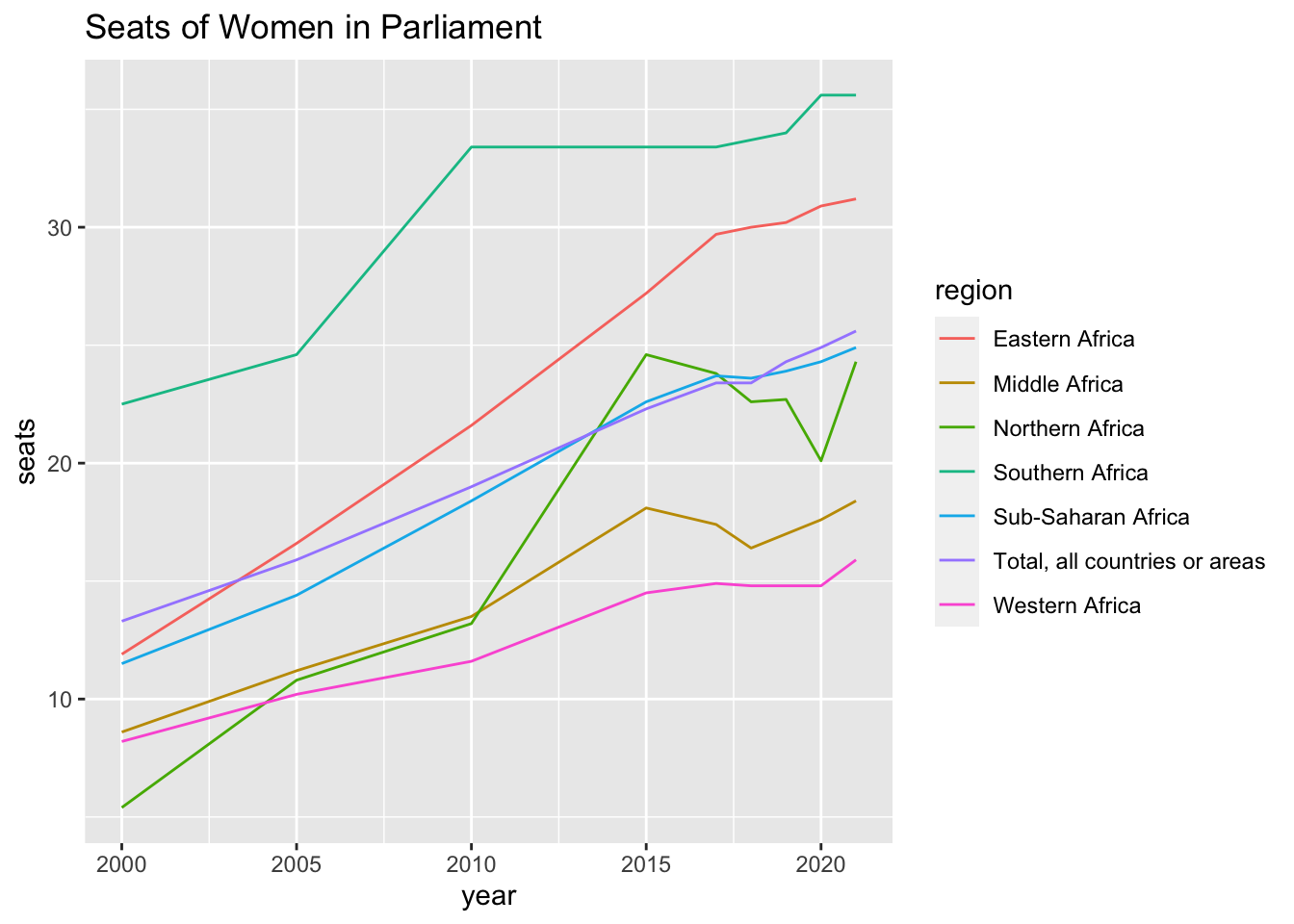

Good Luck!

If you need help, please drop me a line. I would set up a Zoom Office Hour.

HS