2 R and R Studio

2.1 What is R?

2.1.1 R (programming language), Wikipedia

R is a programming language and free software environment for statistical computing and graphics supported by the R Foundation for Statistical Computing.
The R language is widely used among statisticians and data miners for developing statistical software and data analysis.
A GNU package, the official R software environment is written primarily in C, Fortran, and R itself (thus, it is partially self-hosting) and is freely available under the GNU General Public License.

2.1.2 History of R and more

“R Programming for Data Science” by Roger Peng

2.2 Why R? – Responses by Hadley Wickham

2.2.1 r4ds: R is a great place to start your data science journey because

R is an environment designed from the ground up to support data science.
R is not just a programming language, but it is also an interactive environment for doing data science.
To support interaction, R is a much more flexible language than many of its peers.

2.2.2 Why R today?

When you talk about choosing programming languages, I always say you shouldn’t pick them based on technical merits, but rather pick them based on the community. And I think the R community is like really, really strong, vibrant, free, welcoming, and embraces a wide range of domains. So, if there are like people like you using R, then your life is going to be much easier. That’s the first reason.

Interview: “Advice to Young (and Old) Programmers, H. Wickham”

2.3 What is RStudio? https://posit.com

RStudio is an integrated development environment, or IDE, for R programming.

2.3.1 R Studio (Wikipedia)

RStudio is an integrated development environment (IDE) for R, a programming language for statistical computing and graphics. It is available in two formats: RStudio Desktop is a regular desktop application while RStudio Server runs on a remote server and allows accessing RStudio using a web browser.

2.4 Installation of R and R Studio

2.4.1 R Installation

To download R, go to CRAN, the comprehensive R archive network. CRAN is composed of a set of mirror servers distributed around the world and is used to distribute R and R packages. Don’t try and pick a mirror that’s close to you: instead use the cloud mirror, https://cloud.r-project.org, which automatically figures it out for you.

A new major version of R comes out once a year, and there are 2-3 minor releases each year. It’s a good idea to update regularly.

2.4.2 R Studio Installation

Download and install it from http://www.rstudio.com/download.

RStudio is updated a couple of times a year. When a new version is available, RStudio will let you know.

2.5 R Studio

2.5.1 The First Step

Start R Studio Application
Top Menu: File > New Project > New Directory > New Project > Directory name or Browse the directory and choose the parent directory you want to create the directory

2.5.2 When You Start the Project

Go to the directory you created
Double click _‘Directory Name’.Rproj

Or,

Start R Studio
File > Open Project (or choose from Recent Project)

In this way the working directory of the session is set to the project directory and R can search releted files without difficulty (getwd(), setwd())

2.6 Posit Cloud

RStudio Cloud is a lightweight, cloud-based solution that allows anyone to do, share, teach and learn data science online.

2.6.1 Cloud Free

Up to 15 projects total
1 shared space (5 members and 10 projects max)
15 project hours per month
Up to 1 GB RAM per project
Up to 1 CPU per project
Up to 1 hour background execution time

2.6.2 How to Start Posit Cloud

Go to https://posit.cloud/
Sign Up: top right

Email address or Google account

New Project: Project Name
R Console

2.7 Let’s Get Started

Start RStudio and create a project, or login to Posit Cloud and create a project.

2.7.1 The First Examples

Input the following codes into Console in the left bottom pane.

The first two:

head(cars)
#>   speed dist
#> 1     4    2
#> 2     4   10
#> 3     7    4
#> 4     7   22
#> 5     8   16
#> 6     9   10

str(cars)
#> 'data.frame':    50 obs. of  2 variables:
#>  $ speed: num  4 4 7 7 8 9 10 10 10 11 ...
#>  $ dist : num  2 10 4 22 16 10 18 26 34 17 ...

Two more:

summary(cars)
#>      speed           dist       
#>  Min.   : 4.0   Min.   :  2.00  
#>  1st Qu.:12.0   1st Qu.: 26.00  
#>  Median :15.0   Median : 36.00  
#>  Mean   :15.4   Mean   : 42.98  
#>  3rd Qu.:19.0   3rd Qu.: 56.00  
#>  Max.   :25.0   Max.   :120.00

plot(cars)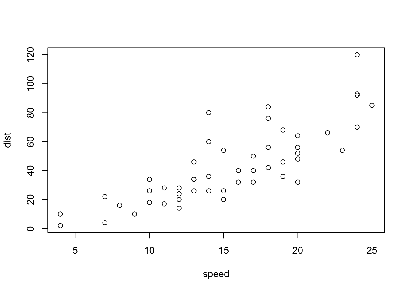

And three more:

plot(cars) # cars: Speed and Stopping Distances of Cars
abline(lm(cars$dist~cars$speed))

lm(cars$dist~cars$speed)
#> 
#> Call:
#> lm(formula = cars$dist ~ cars$speed)
#> 
#> Coefficients:
#> (Intercept)   cars$speed  
#>     -17.579        3.932

summary(lm(cars$dist~cars$speed))
#> 
#> Call:
#> lm(formula = cars$dist ~ cars$speed)
#> 
#> Residuals:
#>     Min      1Q  Median      3Q     Max 
#> -29.069  -9.525  -2.272   9.215  43.201 
#> 
#> Coefficients:
#>             Estimate Std. Error t value Pr(>|t|)    
#> (Intercept) -17.5791     6.7584  -2.601   0.0123 *  
#> cars$speed    3.9324     0.4155   9.464 1.49e-12 ***
#> ---
#> Signif. codes:  
#> 0 '***' 0.001 '**' 0.01 '*' 0.05 '.' 0.1 ' ' 1
#> 
#> Residual standard error: 15.38 on 48 degrees of freedom
#> Multiple R-squared:  0.6511, Adjusted R-squared:  0.6438 
#> F-statistic: 89.57 on 1 and 48 DF,  p-value: 1.49e-12

2.7.1.1 Brief Explanation

cars: A pre-installed data which is a part of package datasets.
head(cars): The first six rows of the pre-installed data cars.
str(cars): The pre-installed data cars data structure.
summary(cars): The summary of the pre-installed data cars.
plot(cars): A scatter plot of the pre-installed data cars.
- plot(cars$dist~cars$speed)
- cars$dist, cars$[[2]], cars[,2] are same
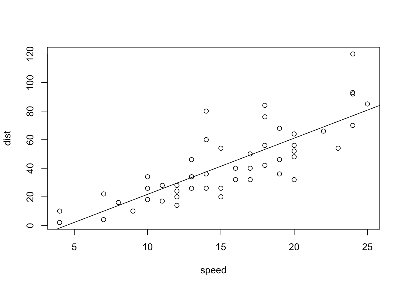
abline(lm(cars$dist~cars$speed)): Add a regression line of a linear model
lm(cars$dist~cars$speed): The equation of the regression line
summary(lm(cars$dist~cars$speed): The summary of the linear regression model

2.7.1.2 Histograms

cars is a data frame consisting of two columns, dist and speed.

hist(cars$dist)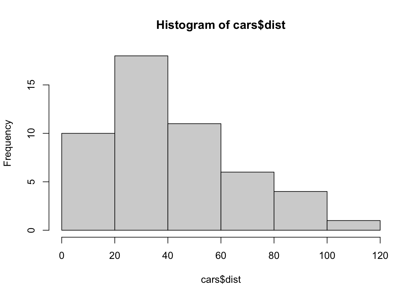

hist(cars$speed)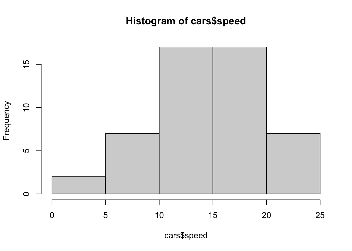

2.7.1.3 View and help

View(cars)
?cars: same as help(cars)
??cars: same as `help.search(“cars”)

2.7.1.4 `datasets`

datasets is a pre-installed datasets which contains a variety of datasets.

?datasets
library(help = "datasets")
data() shows all data already attached and available.

By library(help = "datasets") and/or data(), you can see the complete list of data in datasets.

2.7.2 Practicum

Pick a data in the datasets package and try

and some more.

2.7.3 `iris`

head(iris)
#>   Sepal.Length Sepal.Width Petal.Length Petal.Width Species
#> 1          5.1         3.5          1.4         0.2  setosa
#> 2          4.9         3.0          1.4         0.2  setosa
#> 3          4.7         3.2          1.3         0.2  setosa
#> 4          4.6         3.1          1.5         0.2  setosa
#> 5          5.0         3.6          1.4         0.2  setosa
#> 6          5.4         3.9          1.7         0.4  setosa

str(iris)
#> 'data.frame':    150 obs. of  5 variables:
#>  $ Sepal.Length: num  5.1 4.9 4.7 4.6 5 5.4 4.6 5 4.4 4.9 ...
#>  $ Sepal.Width : num  3.5 3 3.2 3.1 3.6 3.9 3.4 3.4 2.9 3.1 ...
#>  $ Petal.Length: num  1.4 1.4 1.3 1.5 1.4 1.7 1.4 1.5 1.4 1.5 ...
#>  $ Petal.Width : num  0.2 0.2 0.2 0.2 0.2 0.4 0.3 0.2 0.2 0.1 ...
#>  $ Species     : Factor w/ 3 levels "setosa","versicolor",..: 1 1 1 1 1 1 1 1 1 1 ...

summary(iris)
#>   Sepal.Length    Sepal.Width     Petal.Length  
#>  Min.   :4.300   Min.   :2.000   Min.   :1.000  
#>  1st Qu.:5.100   1st Qu.:2.800   1st Qu.:1.600  
#>  Median :5.800   Median :3.000   Median :4.350  
#>  Mean   :5.843   Mean   :3.057   Mean   :3.758  
#>  3rd Qu.:6.400   3rd Qu.:3.300   3rd Qu.:5.100  
#>  Max.   :7.900   Max.   :4.400   Max.   :6.900  
#>   Petal.Width          Species  
#>  Min.   :0.100   setosa    :50  
#>  1st Qu.:0.300   versicolor:50  
#>  Median :1.300   virginica :50  
#>  Mean   :1.199                  
#>  3rd Qu.:1.800                  
#>  Max.   :2.500

Can you plot?

plot(iris$Sepal.Length, iris$Sepal.Width)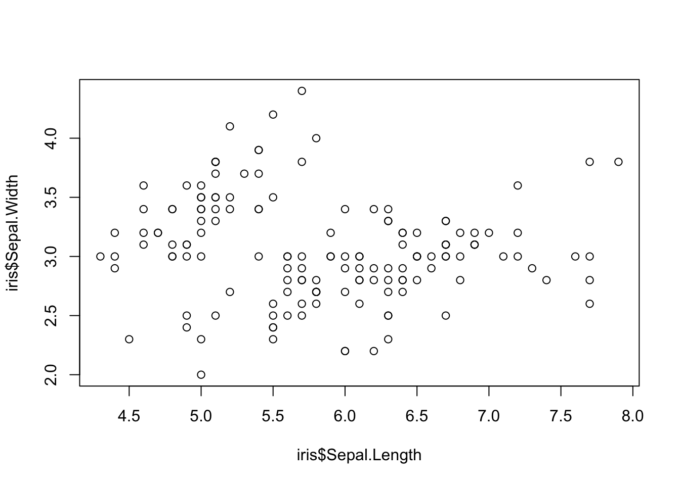

2.8 Brief Introduction to R on RStudio

2.8.1 Create a New Project

After starting RStudio, create a new project using New Project under the top File menu. From next time, you can find your project from Open Project or Recent Project under the top File menu.

You can also start the project by clicking or opening the project_name.Rpoj file.

2.8.2 Four Panes and Tabs

Top Left: Source Editor
Top Right: Environment, History, etc.
Bottom Left: Console, Terminal, Render, Background Jobs
Bottom Right: Files, Plots, Packages, Help, Viewer, Presentation

2.9 Set up

Highly recommend to set the language to be “English”.
Create “data” directory.

Sys.setenv(LANG = "en")
dir.create("./data")

2.10 Three Ways to Run Codes

Console - Bottom Left Pane

We have run codes on the console already!

R Script - pull-down menu under File
R Notebook, R Markdown - pull down menu under File

2.11 R Script - Second Way to Run Codes

2.11.1 Examples: R Scripts in Moodle

basics.R
coronavirus.R

Copy a script in Moodle: {file name}.R
In RStudio (create Project in RStudio) choose File > New File > R Script and paste it.
Choose File > Save As, save with a name; e.g. {file names} (.R will be added automatically)

To run a code: at the cursor press Ctrl+Shift+Enter (Win) or Cmd+Shift+Enter (Mac).

Top Manu: Help > Keyboard Short Cut Help contains many shortcuts.
Bottom Right Pane: Check the files by selecting the Files tab.

2.12 Practicum

Run the following and see what happens. You do not have to understand everything. Please guess what each code does.

2.12.1 R Scripts in Moodle

basics.R
coronavirus.R

Copy a script in Moodle: {file name}.R
In RStudio (Workspace in RStudio.cloud, Project in RStudio) choose File > New File > R Script and paste it.
Choose File > Save with a name; e.g. {file names} (.R will be added automatically)

2.12.2 `basics.R`

The script with the outputs.

#################
#
# basics.R
#
################
# 'Quick R' by DataCamp may be a handy reference: 
#     https://www.statmethods.net/management/index.html
# Cheat Sheet at RStudio: https://www.rstudio.com/resources/cheatsheets/
# Base R Cheat Sheet: https://github.com/rstudio/cheatsheets/raw/main/base-r.pdf
# To execute the line: Control + Enter (Window and Linux), Command + Enter (Mac)
## try your experiments on the console

## calculator

3 + 7

### +, -, *, /, ^ (or **), %%, %/%

3 + 10 / 2

3^2

2^3

2*2*2

### assignment: <-, (=, ->, assign()) 

x <- 5

x 

#### object_name <- value, '<-' shortcut: Alt (option) + '-' (hyphen or minus) 
#### Object names must start with a letter and can only contain letter, numbers, _ and .

this_is_a_long_name <- 5^3

this_is_a_long_name

char_name <- "What is your name?"

char_name

#### Use 'tab completion' and 'up arrow'

### ls(): list of all assignments

ls()
ls.str()

#### check Environment in the upper right pane

### (atomic) vectors

5:10

a <- seq(5,10)

a

b <- 5:10

identical(a,b)

seq(5,10,2) # same as seq(from = 5, to = 10, by = 2)

c1 <- seq(0,100, by = 10)

c2 <- seq(0,100, length.out = 10)

c1

c2

length(c1)

#### ? seq   ? length   ? identical

(die <- 1:6)

zero_one <- c(0,1) # same as 0:1

die + zero_one # c(1,2,3,4,5,6) + c(0,1). re-use

d1 <- rep(1:3,2) # repeat


d1

die == d1

d2 <- as.character(die == d1)

d2

d3 <- as.numeric(die == d1)

d3

### class() for class and typeof() for mode
### class of vectors: numeric, charcters, logical
### types of vectors: doubles, integers, characters, logicals (complex and raw)

typeof(d1); class(d1)

typeof(d2); class(d2)

typeof(d3); class(d3)

sqrt(2)

sqrt(2)^2

sqrt(2)^2 - 2

typeof(sqrt(2))

typeof(2)

typeof(2L)

5 == c(5)

length(5)

### Subsetting

(A_Z <- LETTERS)

A_F <- A_Z[1:6]

A_F

A_F[3]

A_F[c(3,5)]

large <- die > 3

large

even <- die %in% c(2,4,6)

even

A_F[large]

A_F[even]

A_F[die < 4]

### Compare df with df1 <- data.frame(number = die, alphabet = A_F)
df <- data.frame(number = die, alphabet = A_F, stringsAsFactors = FALSE)

df

df$number

df$alphabet

df[3,2]

df[4,1]

df[1]

class(df[1])

class(df[[1]])

identical(df[[1]], die)

identical(df[1],die)

####################
# The First Example
####################

plot(cars)

# Help

? cars

# cars is in the 'datasets' package

data()

# help(cars) does the same as ? cars
# You can use Help tab in the right bottom pane

help(plot)
? par

head(cars)

str(cars)

summary(cars)

x <- cars$speed
y <- cars$dist

min(x)
mean(x)
quantile(x)

plot(cars)

abline(lm(cars$dist ~ cars$speed))

summary(lm(cars$dist ~ cars$speed))

boxplot(cars)

hist(cars$speed)
hist(cars$dist)
hist(cars$dist, breaks = seq(0,120, 10))

2.12.3 coronavirus.R

The script and its outputs. coronavirus.csv is very large

# https://coronavirus.jhu.edu/map.html
# JHU Covid-19 global time series data
# See R pakage coronavirus at: https://github.com/RamiKrispin/coronavirus
# Data taken from: https://github.com/RamiKrispin/coronavirus/tree/master/csv
# Last Updated
Sys.Date()

## Download and read csv (comma separated value) file
coronavirus <- read.csv("https://github.com/RamiKrispin/coronavirus/raw/master/csv/coronavirus.csv")
# write.csv(coronavirus, "data/coronavirus.csv")

## Summaries and structures of the data
head(coronavirus)
str(coronavirus)
coronavirus$date <- as.Date(coronavirus$date)
str(coronavirus)

range(coronavirus$date)
unique(coronavirus$country)
unique(coronavirus$type)

## Set Country
COUNTRY <- "Japan"
df0 <- coronavirus[coronavirus$country == COUNTRY,]
head(df0)
tail(df0)
(pop <- df0$population[1])
df <- df0[c(1,6,7,13)]
str(df)
head(df)
### alternatively,
head(df0[c("date", "type", "cases", "population")])
###

## Set types
df_confirmed <- df[df$type == "confirmed",]
df_death <- df[df$type == "death",]
df_recovery <- df[df$data_type == "recovery",]
head(df_confirmed)
head(df_death)
head(df_recovery)

## Histogram
plot(df_confirmed$date, df_confirmed$cases, type = "h")
plot(df_death$date, df_death$cases, type = "h")
# plot(df_recovered$date, df_recovered$cases, type = "h") # no data for recovery

## Scatter plot and correlation
plot(df_confirmed$cases, df_death$cases, type = "p")
cor(df_confirmed$cases, df_death$cases)


## In addition set a period
start_date <- as.Date("2021-07-01")
end_date <- Sys.Date() 
df_date <- df[df$date >=start_date & df$date <= end_date,]
##

## Set types
df_date_confirmed <- df_date[df_date$type == "confirmed",]
df_date_death <- df_date[df_date$type == "death",]
df_date_recovery <- df_date[df_date$data_type == "recovery",]
head(df_date_confirmed)
head(df_date_death)
head(df_date_recovery)

## Histogram
plot(df_date_confirmed$date, df_date_confirmed$cases, type = "h")
plot(df_date_death$date, df_date_death$cases, type = "h")
# plot(df_date_recovered$date, df_date_recovered$cases, type = "h") # no data for recovery

plot(df_date_confirmed$cases, df_date_death$cases, type = "p")
cor(df_date_confirmed$cases, df_date_death$cases)

### Q0. Change the values of the location and the period and see the outcomes.
### Q1. What is the correlation between df_confirmed$cases and df_death$cases?
### Q2. Do we have a larger correlation value if we shift the dates to implement the time-lag?
### Q3. Do you have any other questions to explore?

#### Extra
plot(df_confirmed$date, df_confirmed$cases, type = "h", 
     main = paste("Comfirmed Cases in",COUNTRY), 
     xlab = "Date", ylab = "Number of Cases")

2.13 Swirl: An interactive learning environment for R and statistics

{swirl} website: https://swirlstats.com
JHU Data Science in coursera uses swirl for exercises.

2.13.1 Swirl Courses

R Programming: The basics of programming in R
Regression Models: The basics of regression modeling in R
Statistical Inference: The basics of statistical inference in R
Exploratory Data Analysis: The basics of exploring data in R

You can install other swirl courses as well

Swirl Courses Organized by Title
Swirl Courses Organized by Author’s Name
Github: swirl courses
- install_course("Course Name Here")

2.13.2 Install and Start Swirl Courses

2.13.2.1 Three Steps to Start Swirl

install.packages("swirl") # Only the first time.
library(swirl) # Everytime you start swirl
swirl() # Everytime you start or resume swirl

2.13.3 R Programming: The basics of programming in R

 1: Basic Building Blocks      2: Workspace and Files     3: Sequences of Numbers    
 4: Vectors                    5: Missing Values          6: Subsetting Vectors      
 7: Matrices and Data Frames   8: Logic                   9: Functions               
10: lapply and sapply         11: vapply and tapply      12: Looking at Data         
13: Simulation                14: Dates and Times        15: Base Graphics

2.13.4 Recommended Sections in Order

1, 3, 4, 5, 6, 7, 12, 15, 14, 8, 9, 10, 11, 13, 2

Section 2 discusses the directories and file systems of a computer
Sections 9, 10, 11 are for programming

2.13.5 Controling a `swirl` Session

… <– That’s your cue to press Enter to continue
You can exit swirl and return to the R prompt (>) at any time by pressing the Esc key.
If you are already at the prompt, type bye() to exit and save your progress. When you exit properly, you’ll see a short message letting you know you’ve done so.

When you are at the R prompt (>):

Typing skip() allows you to skip the current question.
Typing play() lets you experiment with R on your own; swirl will ignore what you do…
UNTIL you type nxt() which will regain swirl’s attention.
Typing bye() causes swirl to exit. Your progress will be saved.
Typing main() returns you to swirl’s main menu.
Typing info() displays these options again.

2.13.6 Final Remarks

You will encounter the message like ‘Would you like to receive credit for completing this course on Coursera.org?’ at the end of each course. This is for coursera courses. Select ‘NO’.

1 About the Course

3 tidyverse