25 Our World in Data

25.1 The package `owidR`

We study the R package owidR for importing data from Our World in Data.

25.2 References

The package official site contains other links. When you quote the package, use the link to the official site.

Package Official Site: https://CRAN.R-project.org/package=owidR
- ReadMe: https://cran.r-project.org/web/packages/owidR/readme/README.html
- Manual: https://cran.r-project.org/web/packages/owidR/owidR.pdf
- Vignette: Create and Analyse a Dataset
owidR: Import Data from Our World in Data
- Man page and source codes

In general, README gives a short introduction to the package, a Manual, the comprehensive descriptions of each function, and a Vignette, a practical introduction containing examples and applications.

25.3 Introduction

This package acts as an interface to Our World in Data datasets, allowing for an easy way to search through data used in over 3,000 charts and load them into the R environment.

25.3.1 Setup

25.3.1.1 Installation

Run the following for the first time

install.packages("owidR")

25.3.1.2 Load the package

library(owidR)
library(tidyverse) 
#> ── Attaching core tidyverse packages ──── tidyverse 2.0.0 ──
#> ✔ dplyr     1.1.2     ✔ readr     2.1.4
#> ✔ forcats   1.0.0     ✔ stringr   1.5.0
#> ✔ ggplot2   3.4.2     ✔ tibble    3.2.1
#> ✔ lubridate 1.9.2     ✔ tidyr     1.3.0
#> ✔ purrr     1.0.1     
#> ── Conflicts ────────────────────── tidyverse_conflicts() ──
#> ✖ dplyr::filter() masks stats::filter()
#> ✖ dplyr::lag()    masks stats::lag()
#> ℹ Use the conflicted package (<http://conflicted.r-lib.org/>) to force all conflicts to become errors

The package automatically load a part of tidyverse, e.g., dplyr, ggplot, …. Since it works well with the schemetidyverse, it is better to load tidyverse with it.

The creator of this package also suggests loading packages plm for panels of data, and texreg for displaying models, but let us start without them until we actually use them. For panel data, see, for example, the site](https://www.aptech.com/blog/introduction-to-the-fundamentals-of-panel-data/).

25.3.2 Core functions

25.3.2.1 List of core functions

In this package, chart is close to data, and chart id is a data indicator.

owid: Get a dataset used in an OWID chart
owid_covid: Get the Our World in Data covid-19 dataset
owid_search: Search the data sources used in OWID charts
owid_source: A function to get source information from an OWID dataset and display it in the R console.
pal_owid: Colour palettes based on the colours used by Our World in Data
view_chart: A function that opens the original OWID chart in your browser
world_map_data: Function that returns a simple feature collection of class sf. Map data is from naturalearthdata.com. Designed to be used internally.

25.3.2.2 Usage

25.3.2.2.1 `owid_search`

Search the data sources used in OWID charts

owid_search(term)

Example

Since the output is long, I cut it off to the first six rows using head().

owid_search("emissions") %>% head()
#>      titles                                                  
#> [1,] "Air pollutant emissions"                               
#> [2,] "Emissions of air pollutants"                           
#> [3,] "Emissions of air pollutants"                           
#> [4,] "Emissions of particulate matter"                       
#> [5,] "Global sulphur dioxide (SO₂) emissions by world region"
#> [6,] "Sulphur dioxide (SO₂) emissions"                       
#>      chart_id                                        
#> [1,] "air-pollutant-emissions"                       
#> [2,] "emissions-of-air-pollutants"                   
#> [3,] "emissions-of-air-pollutants-oecd"              
#> [4,] "emissions-of-particulate-matter"               
#> [5,] "so-emissions-by-world-region-in-million-tonnes"
#> [6,] "so2-emissions"

A matrix is returned. If the list is long, it is easier to see the pairs of the titles and chart_ids by adding as_tibble().

owid_search("emissions") %>% as_tibble()
#> # A tibble: 157 × 2
#>    titles                                           chart_id
#>    <chr>                                            <chr>   
#>  1 Air pollutant emissions                          air-pol…
#>  2 Emissions of air pollutants                      emissio…
#>  3 Emissions of air pollutants                      emissio…
#>  4 Emissions of particulate matter                  emissio…
#>  5 Global sulphur dioxide (SO₂) emissions by world… so-emis…
#>  6 Sulphur dioxide (SO₂) emissions                  so2-emi…
#>  7 Sulphur dioxide (SO₂) emissions                  so-emis…
#>  8 Sulphur dioxide (SO₂) emissions per capita       so-emis…
#>  9 Sulphur oxide (SO₂) emissions                    sulphur…
#> 10 Annual CO2 emissions from land-use change per c… co2-lan…
#> # ℹ 147 more rows

If the list is not long, you do not need to add as_tibble(). However, note that you need to keep in mind that the title and the chart_id consists of a pair, and you need to use the chart_id to download the data using owid.

owid_search("human rights")
#>      titles                                                                             
#> [1,] "Human rights vs. electoral democracy"                                             
#> [2,] "Countries with accredited independent national human rights institutions"         
#> [3,] "Distribution of human rights"                                                     
#> [4,] "Human rights"                                                                     
#> [5,] "Human rights"                                                                     
#> [6,] "Human rights vs. GDP per capita"                                                  
#> [7,] "Number of cases of killed human rights defenders, journalists and trade unionists"
#> [8,] "Share of countries with accredited independent national human rights institutions"
#>      chart_id                                                                   
#> [1,] "human-rights-vs-electoral-democracy"                                      
#> [2,] "countries-with-independent-national-human-rights-institution"             
#> [3,] "distribution-human-rights-vdem"                                           
#> [4,] "human-rights-vdem"                                                        
#> [5,] "human-rights-popw"                                                        
#> [6,] "human-rights-vs-gdp-per-capita"                                           
#> [7,] "cases-of-killed-human-rights-defenders-journalists-trade-unionists"       
#> [8,] "share-countries-accredited-independent-national-human-rights-institutions"

25.3.2.2.2 `owid`

Get a dataset used in an OWID chart

owid(chart_id = NULL, rename = NULL, tidy.date = TRUE, ...)

chard_id: The chart_id as returned by owid_search, which is combined with ‘-’. Don’t mix up with the chart titles.

rename: Rename the value column. Currently only works if their is just one value col- umn.

Example

emissions <- owid("per-capita-ghg-emissions")

emissions
#> # A tibble: 35,646 × 4
#>    entity      code   year Per-capita greenhouse gas emiss…¹
#>  * <chr>       <chr> <int>                             <dbl>
#>  1 Afghanistan AFG    1850                              1.94
#>  2 Afghanistan AFG    1851                              1.96
#>  3 Afghanistan AFG    1852                              1.96
#>  4 Afghanistan AFG    1853                              1.97
#>  5 Afghanistan AFG    1854                              1.97
#>  6 Afghanistan AFG    1855                              1.97
#>  7 Afghanistan AFG    1856                              1.98
#>  8 Afghanistan AFG    1857                              1.98
#>  9 Afghanistan AFG    1858                              1.99
#> 10 Afghanistan AFG    1859                              1.99
#> # ℹ 35,636 more rows
#> # ℹ abbreviated name:
#> #   ¹`Per-capita greenhouse gas emissions in CO2 equivalents`

rights <- owid("human-rights-scores")

rights
#> # A tibble: 11,273 × 4
#>    entity      code   year `Human rights protection`
#>  * <chr>       <chr> <int>                     <dbl>
#>  1 Afghanistan AFG    1946                     0.829
#>  2 Afghanistan AFG    1947                     0.878
#>  3 Afghanistan AFG    1948                     0.935
#>  4 Afghanistan AFG    1949                     0.966
#>  5 Afghanistan AFG    1950                     1.01 
#>  6 Afghanistan AFG    1951                     1.09 
#>  7 Afghanistan AFG    1952                     1.13 
#>  8 Afghanistan AFG    1953                     1.18 
#>  9 Afghanistan AFG    1954                     1.22 
#> 10 Afghanistan AFG    1955                     1.22 
#> # ℹ 11,263 more rows

Note.

You can use rename to change column names. For example,

owid("per-capita-ghg-emissions", rename = "ghgPcap")
#> # A tibble: 35,646 × 4
#>    entity      code   year ghgPcap
#>  * <chr>       <chr> <int>   <dbl>
#>  1 Afghanistan AFG    1850    1.94
#>  2 Afghanistan AFG    1851    1.96
#>  3 Afghanistan AFG    1852    1.96
#>  4 Afghanistan AFG    1853    1.97
#>  5 Afghanistan AFG    1854    1.97
#>  6 Afghanistan AFG    1855    1.97
#>  7 Afghanistan AFG    1856    1.98
#>  8 Afghanistan AFG    1857    1.98
#>  9 Afghanistan AFG    1858    1.99
#> 10 Afghanistan AFG    1859    1.99
#> # ℹ 35,636 more rows

Since until after importing the data, you never know the original column name, and how many columns are for indicators. It is natural to change column names using dpyr::rename. In the next example, I used Total including LUCF. However, ‘Total including LUCF’ and “Total including LUCF” work as well.

emissions %>% rename(ghgPcap = `Per-capita greenhouse gas emissions in CO2 equivalents`)
#> # A tibble: 35,646 × 4
#>    entity      code   year ghgPcap
#>  * <chr>       <chr> <int>   <dbl>
#>  1 Afghanistan AFG    1850    1.94
#>  2 Afghanistan AFG    1851    1.96
#>  3 Afghanistan AFG    1852    1.96
#>  4 Afghanistan AFG    1853    1.97
#>  5 Afghanistan AFG    1854    1.97
#>  6 Afghanistan AFG    1855    1.97
#>  7 Afghanistan AFG    1856    1.98
#>  8 Afghanistan AFG    1857    1.98
#>  9 Afghanistan AFG    1858    1.99
#> 10 Afghanistan AFG    1859    1.99
#> # ℹ 35,636 more rows

If there are more than one variables to rename, use vector notation as follows. Here top_n(1) is same as slice(1), and gives the first row only.

owid("electoral-democracy") %>% top_n(1)
#> Selecting by electdem_vdem_low_owid
#> # A tibble: 3 × 6
#>   entity  code   year `Electoral democracy`
#>   <chr>   <chr> <int>                 <dbl>
#> 1 Denmark DNK    2008                 0.922
#> 2 Denmark DNK    2009                 0.922
#> 3 Denmark DNK    2010                 0.922
#> # ℹ 2 more variables: electdem_vdem_high_owid <dbl>,
#> #   electdem_vdem_low_owid <dbl>

owid("electoral-democracy", rename = c("electoral_democracy", "vdem_high", "vdem_low"))
#> # A tibble: 32,518 × 6
#>    entity code   year electoral_democracy vdem_high vdem_low
#>  * <chr>  <chr> <int>               <dbl>     <dbl>    <dbl>
#>  1 Afgha… AFG    1789               0.019     0.024     0.01
#>  2 Afgha… AFG    1790               0.019     0.024     0.01
#>  3 Afgha… AFG    1791               0.019     0.024     0.01
#>  4 Afgha… AFG    1792               0.019     0.024     0.01
#>  5 Afgha… AFG    1793               0.019     0.024     0.01
#>  6 Afgha… AFG    1794               0.019     0.024     0.01
#>  7 Afgha… AFG    1795               0.019     0.024     0.01
#>  8 Afgha… AFG    1796               0.019     0.024     0.01
#>  9 Afgha… AFG    1797               0.019     0.024     0.01
#> 10 Afgha… AFG    1798               0.019     0.024     0.01
#> # ℹ 32,508 more rows

You can use dplyr::rename, and keep the record of renaming column names.

(democracy <- owid("electoral-democracy"))
#> # A tibble: 32,518 × 6
#>    entity      code   year `Electoral democracy`
#>  * <chr>       <chr> <int>                 <dbl>
#>  1 Afghanistan AFG    1789                 0.019
#>  2 Afghanistan AFG    1790                 0.019
#>  3 Afghanistan AFG    1791                 0.019
#>  4 Afghanistan AFG    1792                 0.019
#>  5 Afghanistan AFG    1793                 0.019
#>  6 Afghanistan AFG    1794                 0.019
#>  7 Afghanistan AFG    1795                 0.019
#>  8 Afghanistan AFG    1796                 0.019
#>  9 Afghanistan AFG    1797                 0.019
#> 10 Afghanistan AFG    1798                 0.019
#> # ℹ 32,508 more rows
#> # ℹ 2 more variables: electdem_vdem_high_owid <dbl>,
#> #   electdem_vdem_low_owid <dbl>

democracy <- democracy %>% 
  rename(`electoral_democracy` = `Electoral democracy`,  
         `vdem_high` = `electdem_vdem_high_owid`, 
         `electdem_vdem_low_owid` = `electdem_vdem_low_owid`)
democracy
#> # A tibble: 32,518 × 6
#>    entity      code   year electoral_democracy vdem_high
#>  * <chr>       <chr> <int>               <dbl>     <dbl>
#>  1 Afghanistan AFG    1789               0.019     0.024
#>  2 Afghanistan AFG    1790               0.019     0.024
#>  3 Afghanistan AFG    1791               0.019     0.024
#>  4 Afghanistan AFG    1792               0.019     0.024
#>  5 Afghanistan AFG    1793               0.019     0.024
#>  6 Afghanistan AFG    1794               0.019     0.024
#>  7 Afghanistan AFG    1795               0.019     0.024
#>  8 Afghanistan AFG    1796               0.019     0.024
#>  9 Afghanistan AFG    1797               0.019     0.024
#> 10 Afghanistan AFG    1798               0.019     0.024
#> # ℹ 32,508 more rows
#> # ℹ 1 more variable: electdem_vdem_low_owid <dbl>

25.3.2.2.3 `owid_source`

A function to get source information from an OWID dataset and display it in the R console.

owid_source(data)

Example

owid_source(emissions)
#> Dataset Name: Our World in Data based on Jones et al. (2023)
#> 
#> Published By: Our World in Data based on Jones, Matthew W., Peters, Glen P., Gasser, Thomas, Andrew, Robbie M., Schwingshackl, Clemens, Gütschow, Johannes, Houghton, Richard A., Friedlingstein, Pierre, Pongratz, Julia, & Le Quéré, Corinne. (2023). National contributions to climate change due to historical emissions of carbon dioxide, methane and nitrous oxide [Data set]. In Scientific Data (2023.1). Zenodo.
#> 
#> 
#> Link: https://zenodo.org/record/7636699#.ZFCy4exBweZ
#> 
#> Jones et al. (2023) quantify national and regional contributions to the increase of global mean surface temperature over the last few centuries.
#> 
#> Original dataset description by Jones et al. (2023):
#> A dataset describing the global warming response to national emissions CO2, CH4 and N2O from fossil and land use sources during 1851-2021.
#> 
#> National CO2 emissions data are collated from the Global Carbon Project (Andrew and Peters, 2022; Friedlingstein et al., 2022). 
#> 
#> National CH4 and N2O emissions data are collated from PRIMAP-hist (HISTTP) (Gütschow et al., 2022).
#> 
#> We construct a time series of cumulative CO2-equivalent emissions for each country, gas, and emissions source (fossil or land use). Emissions of CH4 and N2O emissions are related to cumulative CO2-equivalent emissions using the Global Warming Potential (GWP*) approach, with best-estimates of the coefficients taken from the IPCC AR6 (Forster et al., 2021).
#> 
#> Warming in response to cumulative CO2-equivalent emissions is estimated using the transient climate response to cumulative carbon emissions (TCRE) approach, with best-estimate value of TCRE taken from the IPCC AR6 (Forster et al., 2021, Canadell et al., 2021). 'Warming' is specifically the change in global mean surface temperature (GMST).

owid_source(rights)
#> Dataset Name: Fariss et al. (2020)
#> 
#> Published By:  Fariss CJ, Kenwick MR, Reuning K. Estimating one-sided-killings from a robust measurement model of human rights. Journal of Peace Research. 2020;57(6):801-814. doi:10.1177/0022343320965670
#> 
#> Link: https://dataverse.harvard.edu/dataset.xhtml?persistentId=doi:10.7910/DVN/RQ85GK
#> 
#> This dataset provides the human rights protection scores by Fariss et al. (2020), first developed by Schnakenberg and Fariss (2014).
#> 
#> You can download the code and complete dataset, including supplementary variables, from GitHub: https://github.com/owid/notebooks/tree/main/BastianHerre/human_rights

25.3.2.2.4 `view_chart`

A function that opens the original OWID chart in your browser

view_chart(x)

x Either a tibble returned by owid(), or a chart_id.
Example

The first one uses the chart, i.e., the tibble returned by owid(), and the second, chart_id. You can also embed in your R Markdown file by copying Embed iframe clink from Share botton at the bottom right corner.

firearm_suicide <- owid("suicide-rate-by-firearm")
    view_chart(firearm_suicide)

view_chart("electoral-democracy")

view_chart("share-of-individuals-using-the-internet")

25.3.2.2.5 `pal_owid`

Colour palettes based on the colours used by Our World in Data

25.3.2.2.6 `owid_covid`

owid_covid: Get the Our World in Data covid-19 dataset

owid_covid()

See the detail at the GitHub site.

Example

covid <- owid_covid()

covid %>% filter(location == "Japan")
#> # A tibble: 1,224 × 67
#>    iso_code continent location date       total_cases
#>    <chr>    <chr>     <chr>    <date>           <dbl>
#>  1 JPN      Asia      Japan    2020-01-03          NA
#>  2 JPN      Asia      Japan    2020-01-04          NA
#>  3 JPN      Asia      Japan    2020-01-05          NA
#>  4 JPN      Asia      Japan    2020-01-06          NA
#>  5 JPN      Asia      Japan    2020-01-07          NA
#>  6 JPN      Asia      Japan    2020-01-08          NA
#>  7 JPN      Asia      Japan    2020-01-09          NA
#>  8 JPN      Asia      Japan    2020-01-10          NA
#>  9 JPN      Asia      Japan    2020-01-11          NA
#> 10 JPN      Asia      Japan    2020-01-12          NA
#> # ℹ 1,214 more rows
#> # ℹ 62 more variables: new_cases <dbl>,
#> #   new_cases_smoothed <dbl>, total_deaths <dbl>,
#> #   new_deaths <dbl>, new_deaths_smoothed <dbl>,
#> #   total_cases_per_million <dbl>,
#> #   new_cases_per_million <dbl>,
#> #   new_cases_smoothed_per_million <dbl>, …

25.4 Examples

The following is based on the presentation and the first two R Notebook files created by Professor Kaizoji.

25.4.1 Human Rights- modified from README

Lets use the core functions to get data on how human rights have changed over time. First by searching for charts on human rights.

owid_search("human rights") %>% as_tibble()
#> # A tibble: 8 × 2
#>   titles                                            chart_id
#>   <chr>                                             <chr>   
#> 1 Human rights vs. electoral democracy              human-r…
#> 2 Countries with accredited independent national h… countri…
#> 3 Distribution of human rights                      distrib…
#> 4 Human rights                                      human-r…
#> 5 Human rights                                      human-r…
#> 6 Human rights vs. GDP per capita                   human-r…
#> 7 Number of cases of killed human rights defenders… cases-o…
#> 8 Share of countries with accredited independent n… share-c…

Let’s use the human rights protection dataset.

rights <- owid("human-rights-protection")
rights
#> # A tibble: 11,273 × 4
#>    entity      code   year `Human rights protection`
#>  * <chr>       <chr> <int>                     <dbl>
#>  1 Afghanistan AFG    1946                     0.829
#>  2 Afghanistan AFG    1947                     0.878
#>  3 Afghanistan AFG    1948                     0.935
#>  4 Afghanistan AFG    1949                     0.966
#>  5 Afghanistan AFG    1950                     1.01 
#>  6 Afghanistan AFG    1951                     1.09 
#>  7 Afghanistan AFG    1952                     1.13 
#>  8 Afghanistan AFG    1953                     1.18 
#>  9 Afghanistan AFG    1954                     1.22 
#> 10 Afghanistan AFG    1955                     1.22 
#> # ℹ 11,263 more rows

ggplot2 makes it easy to visualise our data.

rights %>% 
  filter(entity %in% c("United Kingdom", "France", "United States", "Japan")) %>%  
  ggplot(aes(year, `Human rights protection`, colour = entity)) +
  geom_line()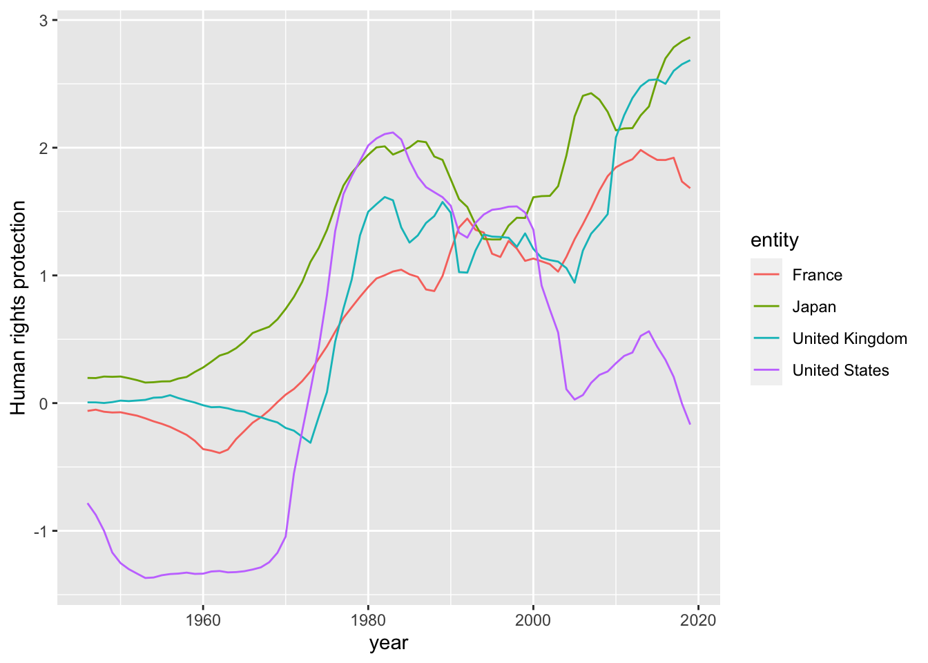

25.4.2 Internet - modified from vignette

owid_search("internet") %>% as_tibble()
#> # A tibble: 7 × 2
#>   titles                                            chart_id
#>   <chr>                                             <chr>   
#> 1 Share of primary schools with access to the Inte… primary…
#> 2 Landline Internet subscriptions                   landlin…
#> 3 Landline Internet subscriptions by download speed landlin…
#> 4 Landline Internet subscriptions per 100 people    broadba…
#> 5 Number of people using the Internet               number-…
#> 6 Share of US adults who use the Internet, by age   share-u…
#> 7 Share of the population using the Internet        share-o…

Get a dataset used in an OWID chart.

owid("share-of-individuals-using-the-internet") %>% top_n(1)
#> Selecting by Individuals using the Internet (% of
#> population)
#> # A tibble: 1 × 4
#>   entity               code   year Individuals using the I…¹
#>   <chr>                <chr> <int>                     <dbl>
#> 1 United Arab Emirates ARE    2020                       100
#> # ℹ abbreviated name:
#> #   ¹`Individuals using the Internet (% of population)`

internet <- owid("share-of-individuals-using-the-internet", rename = "internet_use")
internet
#> # A tibble: 6,660 × 4
#>    entity      code   year internet_use
#>  * <chr>       <chr> <int>        <dbl>
#>  1 Afghanistan AFG    1990      0      
#>  2 Afghanistan AFG    1991      0      
#>  3 Afghanistan AFG    1992      0      
#>  4 Afghanistan AFG    1993      0      
#>  5 Afghanistan AFG    1994      0      
#>  6 Afghanistan AFG    1995      0      
#>  7 Afghanistan AFG    2001      0.00472
#>  8 Afghanistan AFG    2002      0.00456
#>  9 Afghanistan AFG    2003      0.0879 
#> 10 Afghanistan AFG    2004      0.106  
#> # ℹ 6,650 more rows

Get source information on an OWID dataset

owid_source(internet)
#> Dataset Name: International Telecommunication Union (via World Bank)
#> 
#> Published By: World Development Indicators - World Bank (2022.05.26)
#> 
#> Link: https://datacatalog.worldbank.org/search/dataset/0037712/World-Development-Indicators

A function that opens the original OWID chart in your browser.

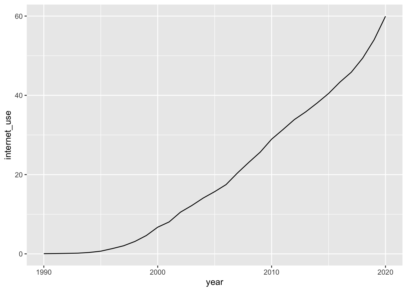
view_chart(internet)

Plot an owid dataset. The first is the simplest, and the second uses oied theme.

internet %>% filter(entity == "World") %>%
  ggplot(aes(year, internet_use))+ geom_line()

internet %>% filter(entity == "World") %>%
  ggplot(aes(year, internet_use))+ geom_line() +
  labs(title = "Share of the World Population \nusing the Internet",
       y = "Individuals using the Internet \n(% of population)") +
  scale_y_continuous(limits = c(0, 100))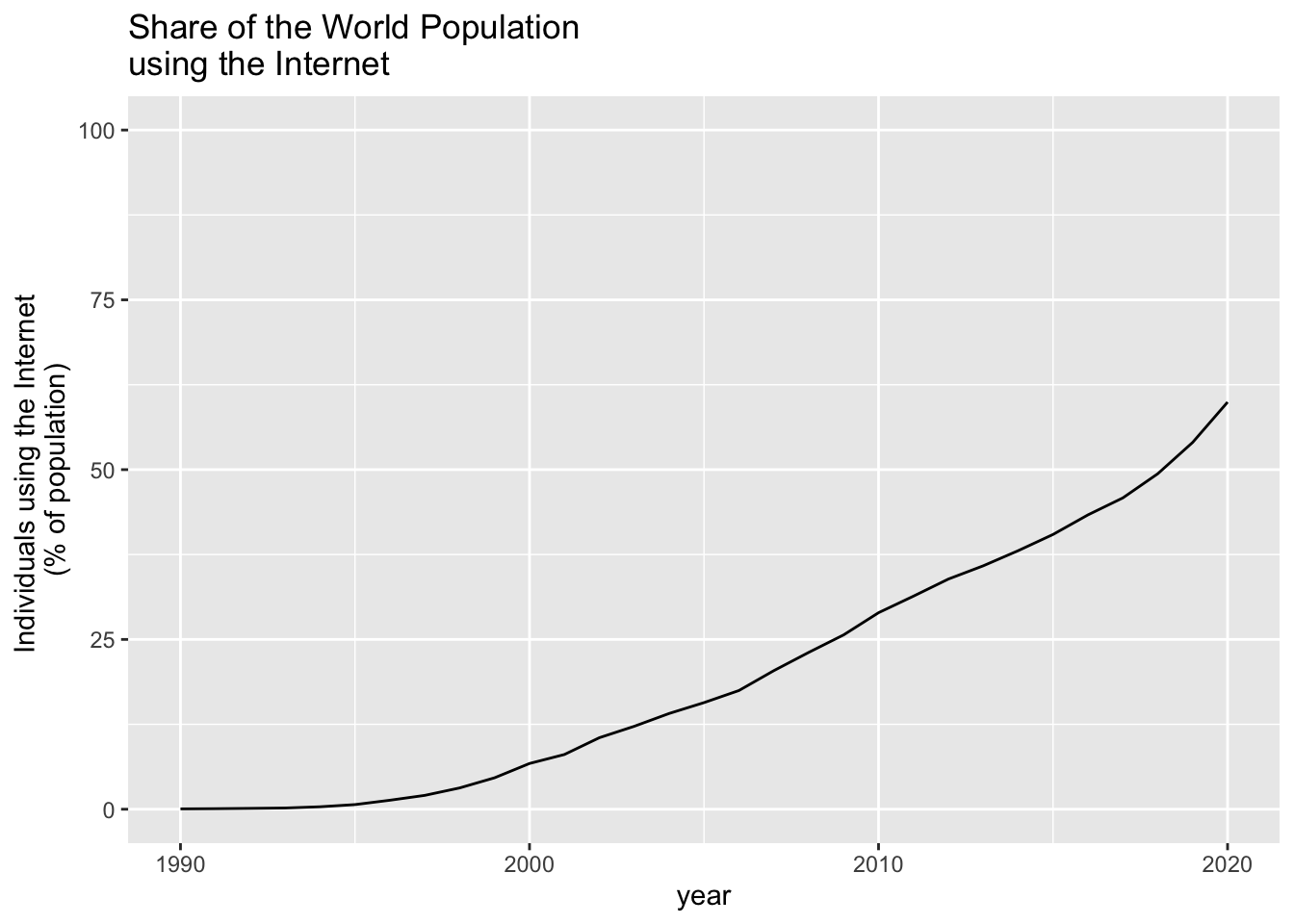

internet %>% 
  filter(entity %in% c("United Kingdom", "Spain", "Russia", "Egypt", "Nigeria")) %>% 
  ggplot(aes(year, internet_use, color =  entity)) + geom_line() +
  labs(title = "Share of Population with Using the Internet",
       y = "Individuals using the Internet \n(% of population)",
       color = "country") +
  scale_y_continuous(limits = c(0, 100), labels = scales::label_number(suffix = "%"))

Creating a choropleth map.

owid_map(internet, year = 2017) +
  labs(title = "Share of Population Using the Internet, 2017")
#> Warning: `owid_map()` was deprecated in owidR 1.4.0.
#> ℹ Please use `ggplot2::ggplot()` instead.
#> This warning is displayed once every 8 hours.
#> Call `lifecycle::last_lifecycle_warnings()` to see where
#> this warning was generated.
#> Warning: `theme_owid()` was deprecated in owidR 1.4.0.
#> ℹ Please use `ggplot2::theme()` instead.
#> ℹ The deprecated feature was likely used in the owidR
#>   package.
#>   Please report the issue to the authors.
#> This warning is displayed once every 8 hours.
#> Call `lifecycle::last_lifecycle_warnings()` to see where
#> this warning was generated.
#> Loading required namespace: showtext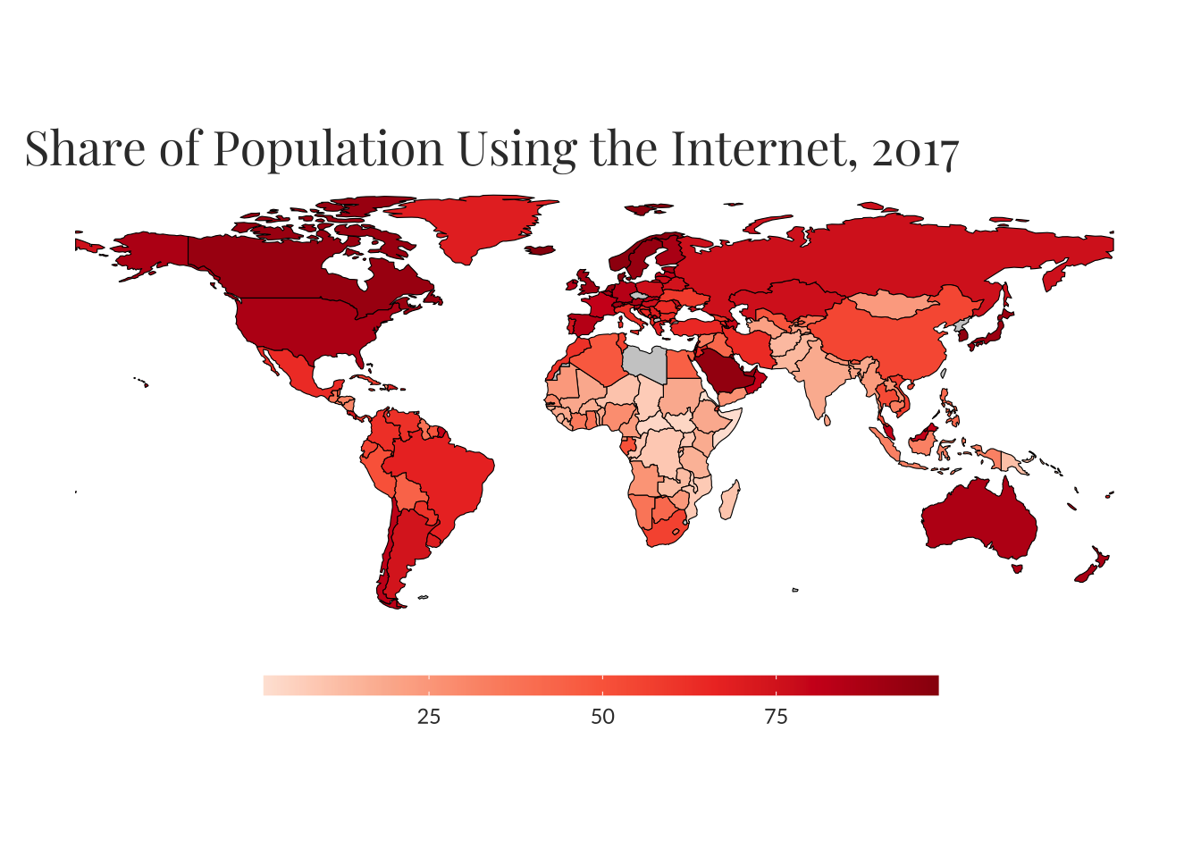

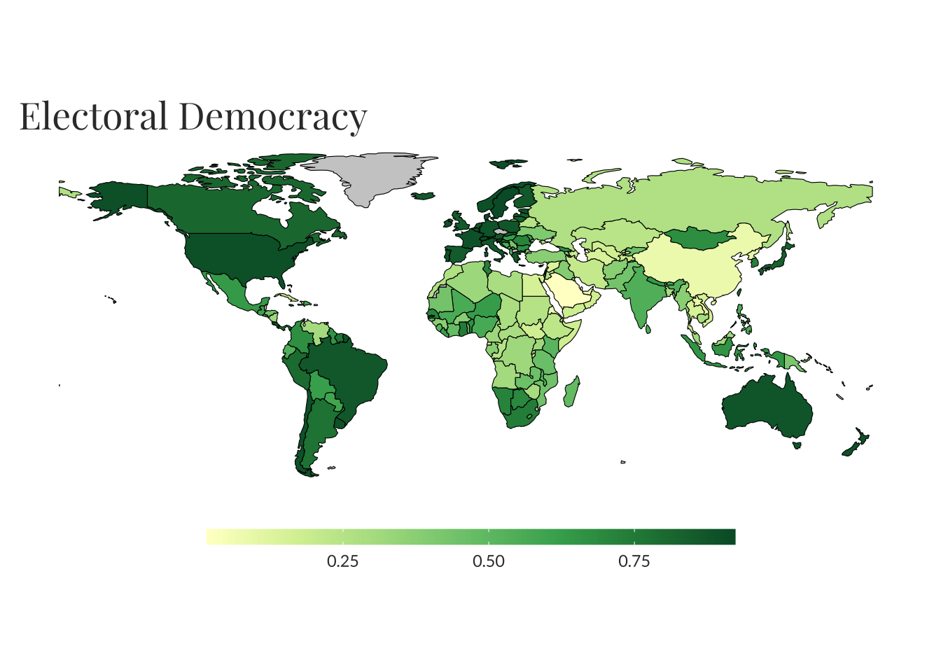
25.4.3 Democracy - modified from vignette

owid_search("democrac") %>% as_tibble()
#> # A tibble: 91 × 2
#>    titles                                           chart_id
#>    <chr>                                            <chr>   
#>  1 Child mortality rate vs. electoral democracy     child-m…
#>  2 People living in democracies and non-democracies world-p…
#>  3 Age of democracy                                 age-of-…
#>  4 Age of democracy                                 age-of-…
#>  5 Age of democracy                                 age-of-…
#>  6 Age of electoral democracy                       age-of-…
#>  7 Age of electoral democracy                       age-of-…
#>  8 Age of liberal democracy                         age-of-…
#>  9 Citizen satisfaction with democracy              citizen…
#> 10 Citizen support for democracy                    citizen…
#> # ℹ 81 more rows

owid("electoral-democracy") %>% top_n(1)
#> Selecting by electdem_vdem_low_owid
#> # A tibble: 3 × 6
#>   entity  code   year `Electoral democracy`
#>   <chr>   <chr> <int>                 <dbl>
#> 1 Denmark DNK    2008                 0.922
#> 2 Denmark DNK    2009                 0.922
#> 3 Denmark DNK    2010                 0.922
#> # ℹ 2 more variables: electdem_vdem_high_owid <dbl>,
#> #   electdem_vdem_low_owid <dbl>

democracy <- owid("electoral-democracy", rename = c("electoral_democracy", "vdem_high", "vdem_low"))
democracy
#> # A tibble: 32,518 × 6
#>    entity code   year electoral_democracy vdem_high vdem_low
#>  * <chr>  <chr> <int>               <dbl>     <dbl>    <dbl>
#>  1 Afgha… AFG    1789               0.019     0.024     0.01
#>  2 Afgha… AFG    1790               0.019     0.024     0.01
#>  3 Afgha… AFG    1791               0.019     0.024     0.01
#>  4 Afgha… AFG    1792               0.019     0.024     0.01
#>  5 Afgha… AFG    1793               0.019     0.024     0.01
#>  6 Afgha… AFG    1794               0.019     0.024     0.01
#>  7 Afgha… AFG    1795               0.019     0.024     0.01
#>  8 Afgha… AFG    1796               0.019     0.024     0.01
#>  9 Afgha… AFG    1797               0.019     0.024     0.01
#> 10 Afgha… AFG    1798               0.019     0.024     0.01
#> # ℹ 32,508 more rows

owid_source(democracy)
#> Value:  
#> 
#> Dataset Name: OWID based on V-Dem (v13) and Lührmann et al. (2018)
#> 
#> Published By: Our World in Data, Bastian Herre
#> 
#> Link: http://v-dem.net/vdemds.html
#> 
#> This dataset provides information on democracy and human rights, using data from the Varieties of Democracy project (v12), and the Regimes of the World classification by Lührmann et al. (2018).
#> 
#> We expand the countries and years covered, and refine the coding of the Regimes of the World classification. You can read a detailed description of the data in these posts:
#> https://ourworldindata.org/regimes-of-the-world-data
#> https://ourworldindata.org/vdem-electoral-democracy-data
#> https://ourworldindata.org/vdem-human-rights-data
#> 
#> You can download the code and complete dataset, including supplementary variables, from GitHub: https://github.com/owid/notebooks/tree/main/BastianHerre/democracy
#> Value:  
#> 
#> Dataset Name: OWID based on V-Dem (v13) and Lührmann et al. (2018)
#> 
#> Published By: Our World in Data, Bastian Herre
#> 
#> Link: http://v-dem.net/vdemds.html
#> 
#> This dataset provides information on democracy and human rights, using data from the Varieties of Democracy project (v12), and the Regimes of the World classification by Lührmann et al. (2018).
#> 
#> We expand the countries and years covered, and refine the coding of the Regimes of the World classification. You can read a detailed description of the data in these posts:
#> https://ourworldindata.org/regimes-of-the-world-data
#> https://ourworldindata.org/vdem-electoral-democracy-data
#> https://ourworldindata.org/vdem-human-rights-data
#> 
#> You can download the code and complete dataset, including supplementary variables, from GitHub: https://github.com/owid/notebooks/tree/main/BastianHerre/democracy
#> Value:  
#> 
#> Dataset Name: OWID based on V-Dem (v13) and Lührmann et al. (2018)
#> 
#> Published By: Our World in Data, Bastian Herre
#> 
#> Link: http://v-dem.net/vdemds.html
#> 
#> This dataset provides information on democracy and human rights, using data from the Varieties of Democracy project (v12), and the Regimes of the World classification by Lührmann et al. (2018).
#> 
#> We expand the countries and years covered, and refine the coding of the Regimes of the World classification. You can read a detailed description of the data in these posts:
#> https://ourworldindata.org/regimes-of-the-world-data
#> https://ourworldindata.org/vdem-electoral-democracy-data
#> https://ourworldindata.org/vdem-human-rights-data
#> 
#> You can download the code and complete dataset, including supplementary variables, from GitHub: https://github.com/owid/notebooks/tree/main/BastianHerre/democracy

owid_map(democracy, year = 2015, palette = "YlGn") +
  labs(title = "Electoral Democracy")

democracy %>% 
  filter(entity %in% c("United Kingdom", "Spain", "Russia", "Egypt", "Nigeria")) %>%
  ggplot(aes(year, electoral_democracy, color = entity)) + geom_line() +
  labs(title = "Electoral Democracy", y = "", color = "country") +
  scale_y_continuous(limits = c(0, 1), labels = scales::label_number(suffix = "%"))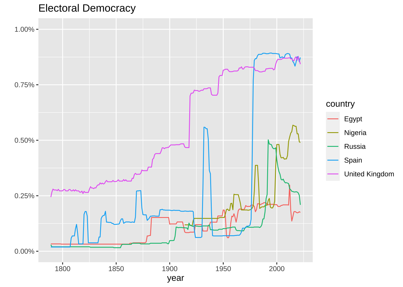

gdp <- owid("gdp-per-capita-worldbank", rename = "gdp")

gov_exp <- owid("total-gov-expenditure-gdp-wdi", rename = "gov_exp")

age_dep <- owid("age-dependency-ratio-of-working-age-population", rename = "age_dep")

unemployment <- owid("unemployment-rate", rename = "unemp")

Mutating joins

left_join(): includes all rows in x.

References

See https://dplyr.tidyverse.org/reference/mutate-joins.html.
Posit Primers - Tidy your data: https://posit.cloud/learn/primers/4
- Join Data Sets: https://posit.cloud/learn/primers/4.3

data <- internet %>% 
  left_join(democracy) %>% 
  left_join(gdp) %>% 
  left_join(gov_exp) %>% 
  left_join(age_dep) %>% 
  left_join(unemployment)
#> Joining with `by = join_by(entity, code, year)`
#> Joining with `by = join_by(entity, code, year)`
#> Joining with `by = join_by(entity, code, year)`
#> Joining with `by = join_by(entity, code, year)`
#> Joining with `by = join_by(entity, code, year)`

Drawing scatter plot

data %>% 
  filter(year == 2015) %>% 
  ggplot(aes(internet_use, electoral_democracy)) +
  geom_point(colour = "#57677D", na.rm = TRUE) +
  geom_smooth(method = "lm", colour = "#DC5E78", na.rm = TRUE) +
  labs(title = "Relationship Between Internet Use \nand electoral_democracy", x = "Internet Use", y = "electoral_democracy")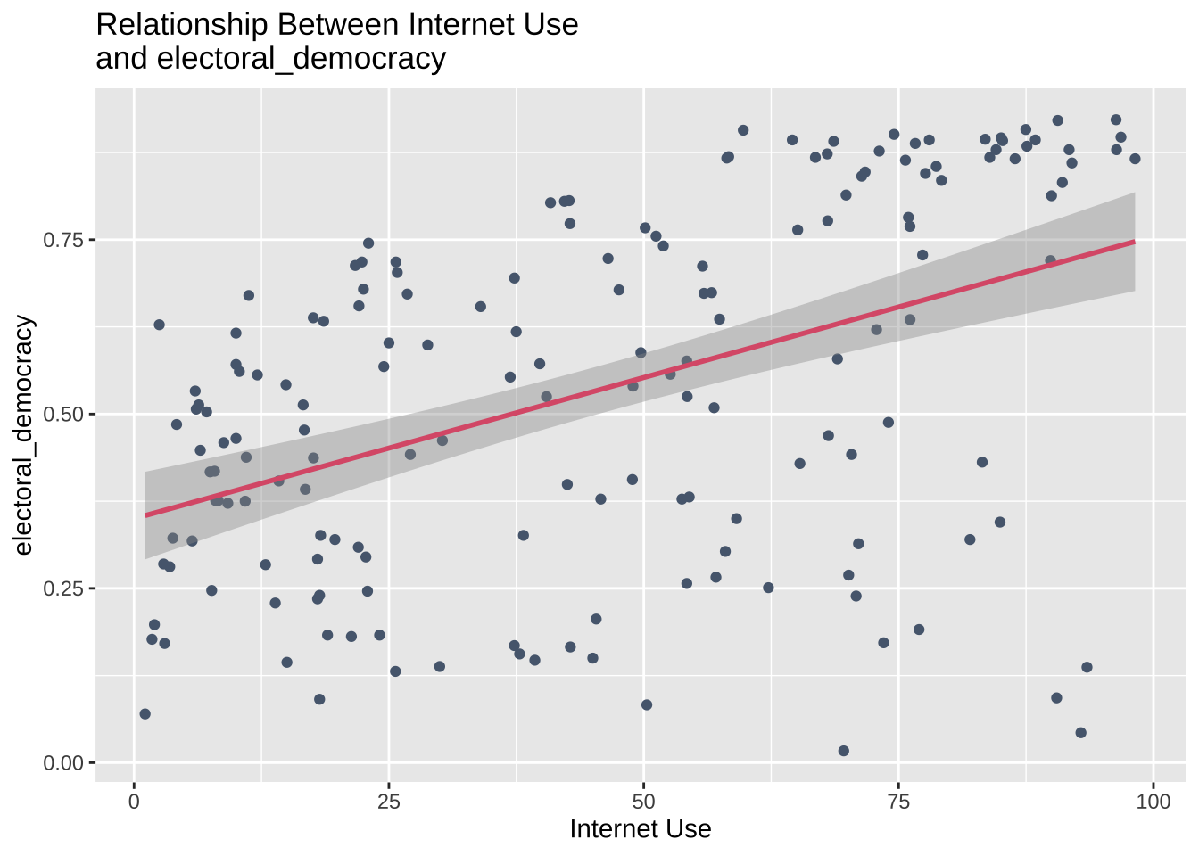

data %>% 
  filter(year == 2015) %>% 
  ggplot(aes(gdp, internet_use)) +
  geom_point(colour = "blue") +
  geom_smooth(method = "gam", colour = "red", level = 0.0) +
  labs(title = "Relationship Between Internet Use and GDP", x = "GDP", y = "Internet Use")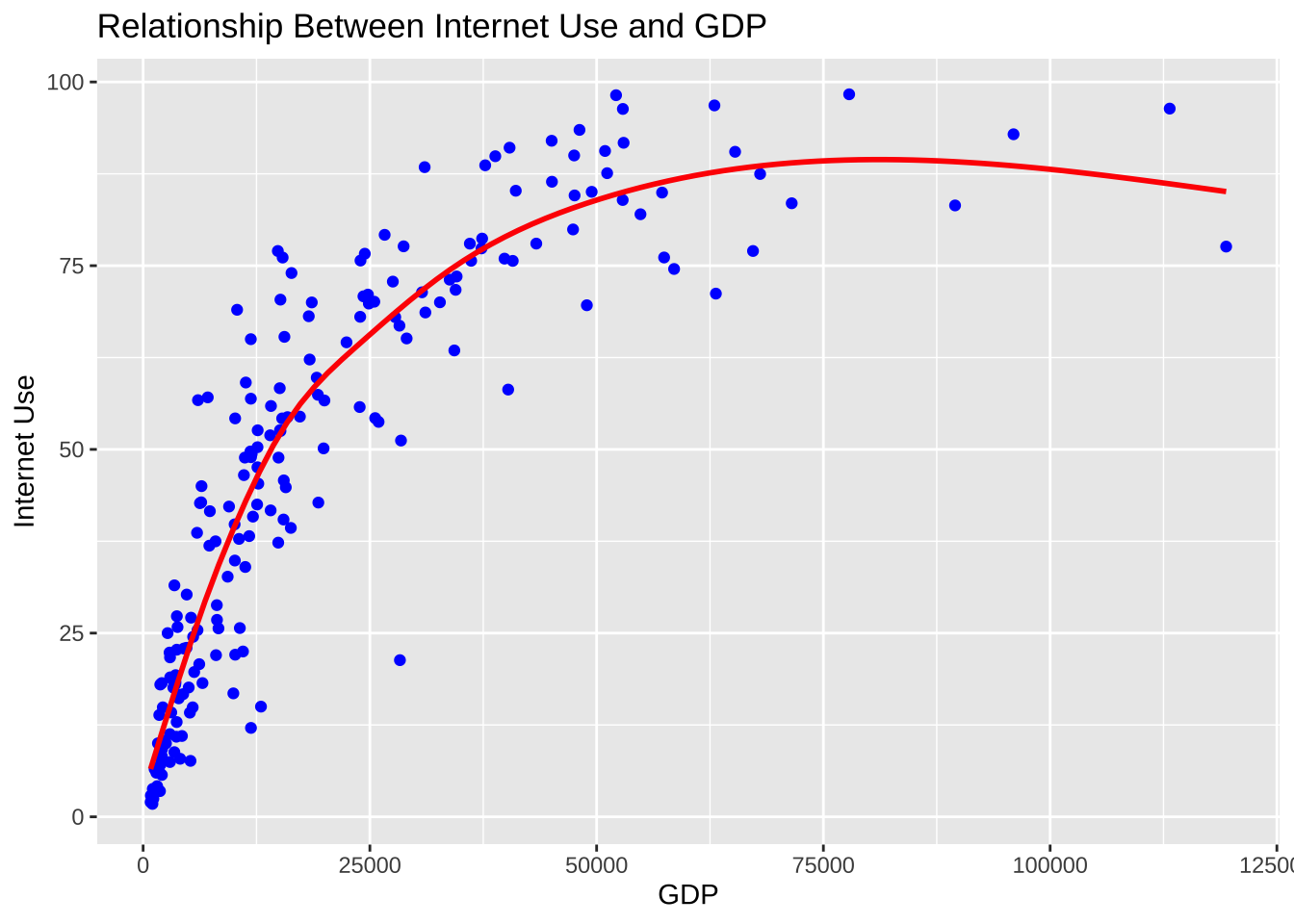

model1 <- lm(electoral_democracy ~ internet_use, data)
summary(model1)
#> 
#> Call:
#> lm(formula = electoral_democracy ~ internet_use, data = data)
#> 
#> Residuals:
#>      Min       1Q   Median       3Q      Max 
#> -0.75942 -0.20190  0.02182  0.18847  0.48518 
#> 
#> Coefficients:
#>               Estimate Std. Error t value Pr(>|t|)    
#> (Intercept)  0.4277459  0.0042857   99.81   <2e-16 ***
#> internet_use 0.0035426  0.0001167   30.36   <2e-16 ***
#> ---
#> Signif. codes:  
#> 0 '***' 0.001 '**' 0.01 '*' 0.05 '.' 0.1 ' ' 1
#> 
#> Residual standard error: 0.2477 on 5311 degrees of freedom
#>   (1347 observations deleted due to missingness)
#> Multiple R-squared:  0.1478, Adjusted R-squared:  0.1477 
#> F-statistic: 921.4 on 1 and 5311 DF,  p-value: < 2.2e-16

model2 <- lm(gdp ~ internet_use, data)
summary(model2)
#> 
#> Call:
#> lm(formula = gdp ~ internet_use, data = data)
#> 
#> Residuals:
#>    Min     1Q Median     3Q    Max 
#> -35872  -7670  -4496   3306 126683 
#> 
#> Coefficients:
#>              Estimate Std. Error t value Pr(>|t|)    
#> (Intercept)  8101.982    276.503   29.30   <2e-16 ***
#> internet_use  413.174      7.315   56.48   <2e-16 ***
#> ---
#> Signif. codes:  
#> 0 '***' 0.001 '**' 0.01 '*' 0.05 '.' 0.1 ' ' 1
#> 
#> Residual standard error: 16350 on 5872 degrees of freedom
#>   (786 observations deleted due to missingness)
#> Multiple R-squared:  0.352,  Adjusted R-squared:  0.3519 
#> F-statistic:  3190 on 1 and 5872 DF,  p-value: < 2.2e-16

Creating a table of the results of the regression analysis using texreg. For the first time, install the pacage texreg.

install.packages("texreg")

library(texreg)
#> Version:  1.38.6
#> Date:     2022-04-06
#> Author:   Philip Leifeld (University of Essex)
#> 
#> Consider submitting praise using the praise or praise_interactive functions.
#> Please cite the JSS article in your publications -- see citation("texreg").
#> 
#> Attaching package: 'texreg'
#> The following object is masked from 'package:tidyr':
#> 
#>     extract

models <- list("Model 1" = model1,
               "Model 2" = model2)
screenreg(models, stars = NULL)
#> 
#> ================================
#>               Model 1   Model 2 
#> --------------------------------
#> (Intercept)      0.43   8101.98 
#>                 (0.00)  (276.50)
#> internet_use     0.00    413.17 
#>                 (0.00)    (7.32)
#> --------------------------------
#> R^2              0.15      0.35 
#> Adj. R^2         0.15      0.35 
#> Num. obs.     5313      5874    
#> ================================

24 World Bank

26 OECD